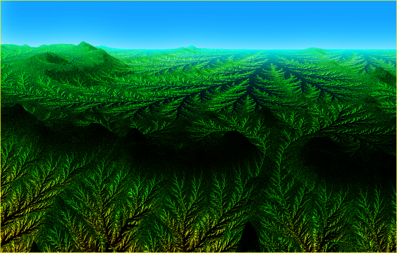
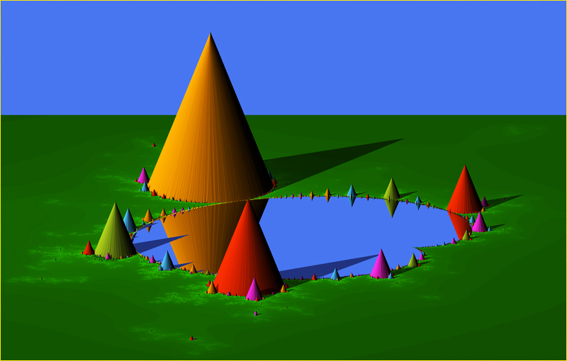
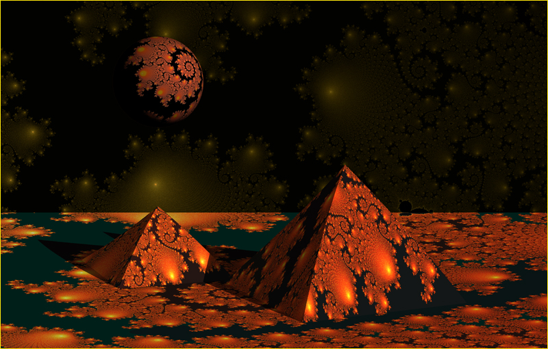
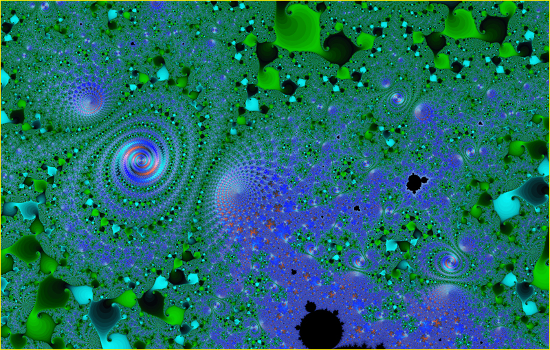
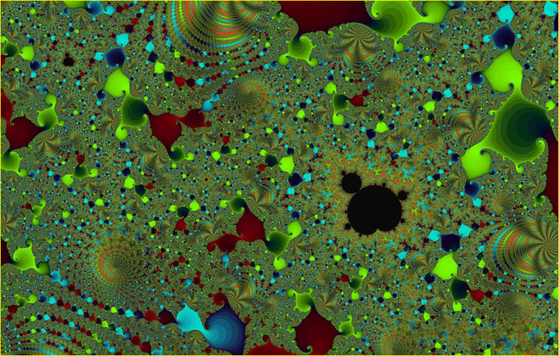
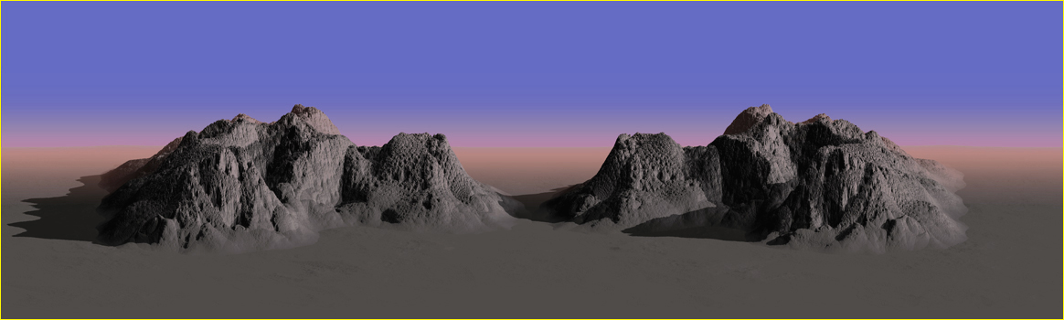
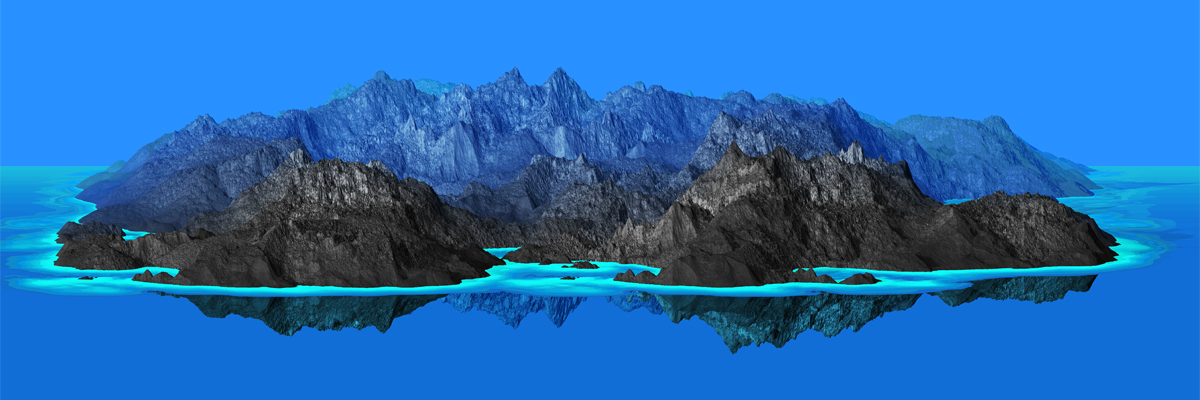
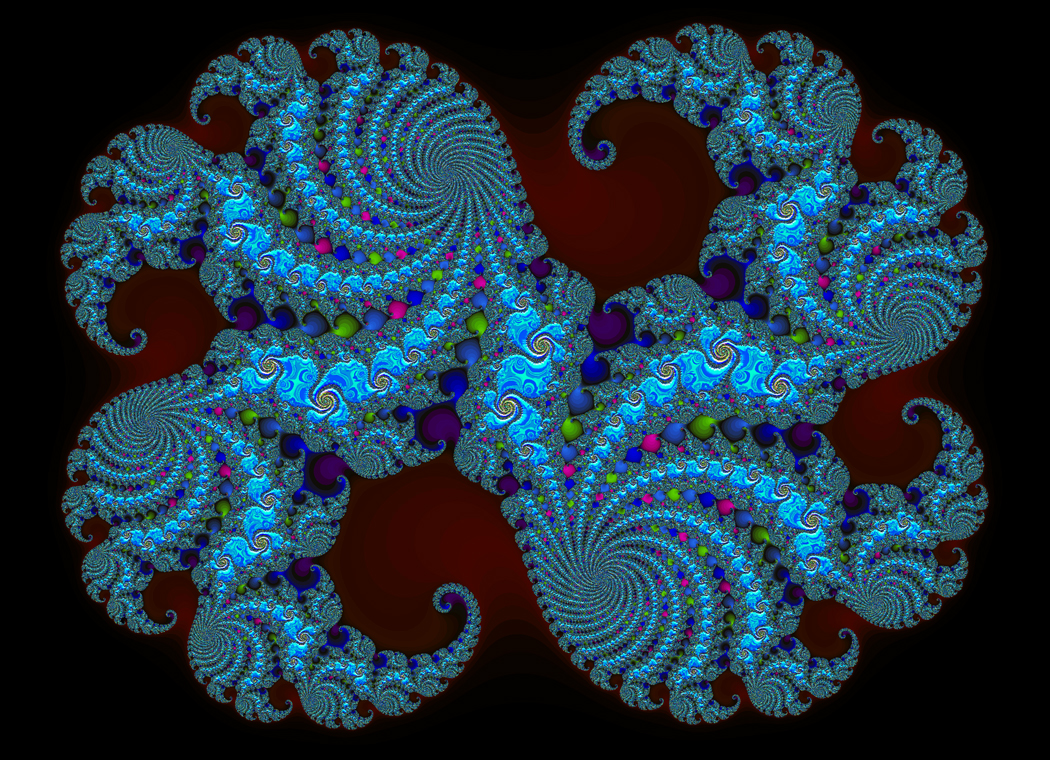
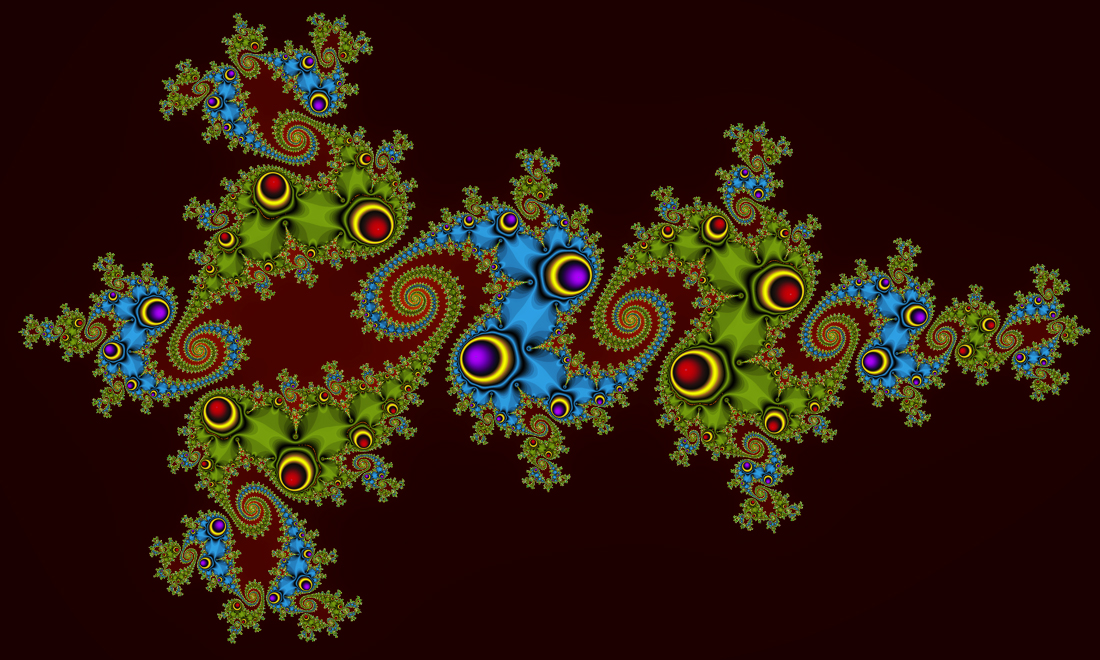
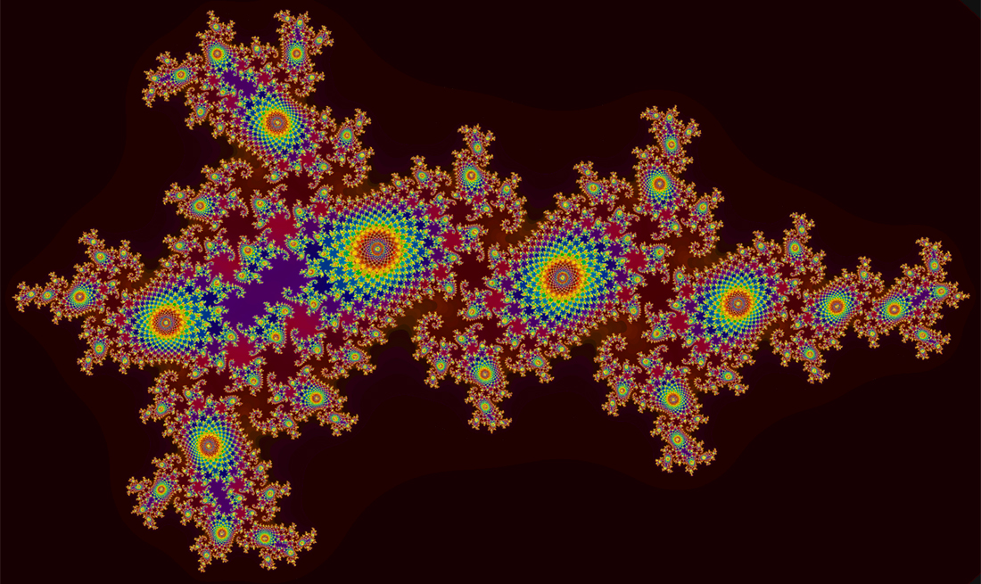
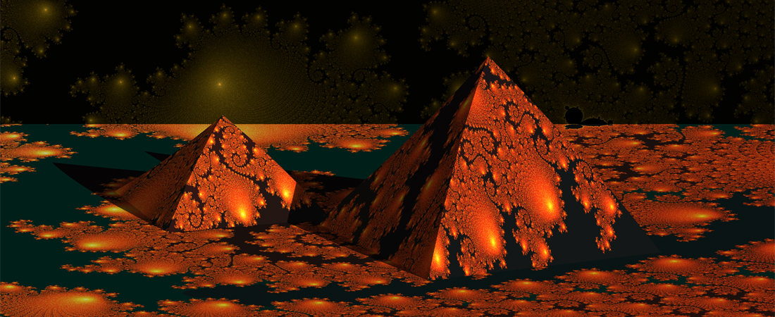
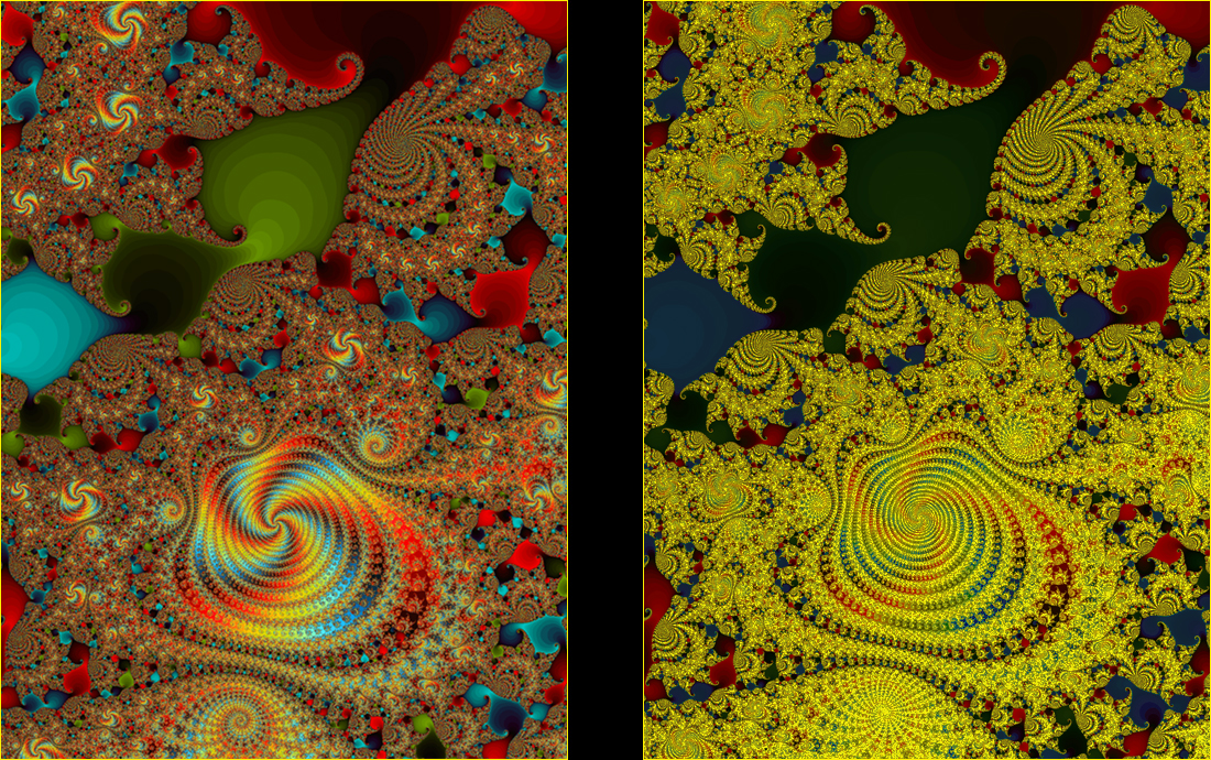
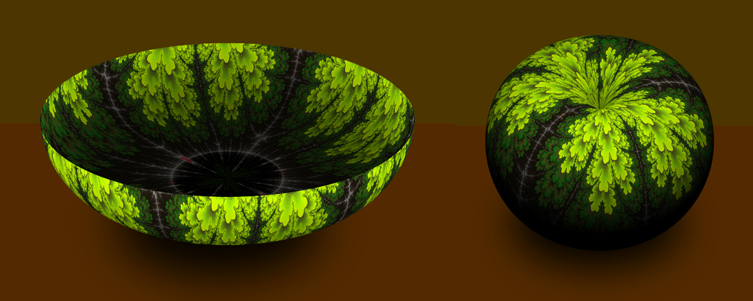
This website is a gallery of computer-generated fractal art as well as a text that explains what it is and how it is created. Central to the website are a myriad of fractal images shown in "Stories about Fractal Art" augmented by the text as optional references. In addition, there are two galleries of fractal art: Gallery 2D is a collection of two-dimensional (2D) images made recently, while Gallery 3D comprises such 3D objects as fractal mountains (some are realistic and others imaginative), fractal forests and fractals painted on various nonplanar surfaces. Here are examples:

 "Symmetric Rocks in Desert"

 "Pyramid" "Escher-like Fern Mountains" 

 "Newton's Apple" "Dragon's Egg" "Broken Taiko Drum" 

 "Copper Bowl" "Antique Vase" 

 "Tamarack Forest"

"Birdless Island" 

and
"Mandelbrot Moon Over Fractal Mountains"


Copyright © 1997-2024 Junpei Sekino 
The website was last updated on March 10, 2024 

Digital Artist (Author's Profile): When Junpei Sekino was 10 years old he won first prize for the junior division in a national printmaking contest in Japan.
He now combines art and mathematics to create fractal art. ...from MathThematics, Book 3, Houghton Mifflin, 1998, 2008.
Stories about Fractal Art
From Art and Mathematics Married by Computer

Contents   Introduction

§ 1. Previews of § 2 - § 8
Prep Math: Orbits, Dynamical Systems and Topological Ideas

§ 2. The Divergence Scheme
§ 3. The Mandelbrot Set
§ 6. Generalizations

Fractal Coloring Algorithms
§ 4. The Convergence Scheme
§ 7. The Logistic Equation

Gallery 2D Gallery 3D
§ 5. Julia Sets
§ 8. Newton Fractals

Sekino's Home Page


Introduction: Speaking loosely without using technical terms such as the Hausdorff-Besicovitch dimension, a fractal is an object that is self-similar, i.e., a large part of it contains smaller parts that resemble the large part in some way; see Figures 0.1-0.5 shown below. Benoit Mandelbrot coined the term "fractal" in 1975 and created a branch of mathematics called fractal geometry seven years later. As an "IBM fellow," he had access to some of the best computers and technical assistants available for his research at the time.
 Figure 0.1. The Mandelbrot Set Figure 0.2.  A Julia Set Figure 0.3. A Newton Fractal 


Our world has fractals everywhere exemplified by trees, mountains, blood vessels, mycelium strands, stock market graphs, weather patterns, seismic rhythms, ECG signals and brain waves. In its article entitled "How Mandelbrot's fractals changed the world," the BBC states that fractal geometry has practical applications in diverse areas including diagnosing some diseases, computer file compression systems and the architecture of the networks that make up the Internet.

The idea of fractal was not particularly new in mathematics for Mandelbrot's time or the computer age, as Georg Cantor introduced the prototypical Cantor set in 1883 and various others appeared as shown in Figure 0.4. In the 1910s, Pierre Fatou and Gaston Julia independently laid the foundations for fractals generated by "dynamical systems" of complex numbers. The Julia sets, representing their fractals and named after Gaston Julia, were largely ignored, however, before the Mandelbrot set was born on a computer screen. The Cantor sets, the Julia sets and the Mandelbrot set are all subsets of the
complex plane.


Figure 0.4. Classical Fractals in Mathematics


Koch Snowflake (1904) Sierpinski Rectangle (1916) Pythagorean Tree (1942)


Sierpinski Triangle (1915) Pascal's Triangles with Modular Arithmetic Devil's Staircase (1884)


It was 1980 when Mandelbrot published his computer-generated image of an object, now called the Mandelbrot set, and completely altered the fate of fractals in mathematics. Mandelbrot, who once studied under Gaston Julia and later became an "IBM fellow," used the computer to visualize the
fundamental dichotomy of the Julia sets, which is a corollary to the Fatou-Julia theorem and divides up the complex plane into two regions.

Thus born was an object that turned out to be astoundingly complex as well as beautiful, unimaginable from the dichotomy. It invigorated the interests in fractals by numerous mathematicians including Adrien Douady and John H. Hubbard, who named the object the "Mandelbrot set" and established many of its properties. Because attractive images of the Mandelbrot set can be generated by a simple computer algorithm, it also found a way out of mathematical communities and into popular culture.

The NOVA program broadcast by PBS in 2008: "Largely because of its haunting beauty, the Mandelbrot set has become the most famous object in modern mathematics. It is also the breeding ground for the world's most famous fractals. Since 1980, the set has provided an inspiration for artists, a source of wonder for schoolchildren, and a fertile testing ground for the science of linear dynamics."


Figure 0.5(A). A Mini-Mandelbrot Set


A Subset of the Mandelbrot Set in Color.
See Figure 3.3 for Detail and Gallery 2D for Applications.


Figure 0.5(B). A Julia Set in Color


Fatou and Julia were born too early to explore computer-generated fractals.


Figure 0.5(C). Another Subset of the Mandelbrot Set in Color


The Mandelbrot set provides a breeding ground for infinitely many fractals including:
Figures 0.5(A)(B)(C)(D), 0.6(C)(D), 0.8(A)(B), 1.0(A)(B)(C), 1.2(B)(G)(H), 1.5(A), 2.0, 2.2, etc., etc.


Figure 0.5(D). A Subset of the Boundary of the Mandelbrot Set


No figures on a plane are more complex than the boundary of the Mandelbrot set.


The late 1970s and the early 1980s were an exciting period for computer lovers as personal computers (PCs) such as Apple II not only became widely available but also grew into major entertainment devices thanks to the arrivals of "Space Invaders" and "Pacman" from Nintendo. A large part of mathematics became experimental like chemistry and physics, as younger mathematicians began to utilize PCs as their research tools. They find clues and solutions by conducting numerical experiments and simulations and it became a trend mainly because of the debuts of "fractal geometry"―and "chaos theory."


Figure 0.6(A). Classical Fractal in Art: Hokusai's "Great Wave off Kanagawa" (1831)


Key Line Art Block Depicting
"Chaotic" Wave of the Sea
Final Woodblock Print
= Key Block + Color Blocks


Figure 0.6(B). Similarities
Between Hokusai's Woodblock Print and Computer-Generated Fractal Art


Chaotic Julia Set
Julia Fractal
= Julia Set + Coloring


in Fractal Geometry in Fractal Art


Chaotic Julia Set
Julia Fractal
= Julia Set + Coloring


in Fractal Geometry in Fractal Art


Figure 0.6(C). "Congregating Owls"


Another Julia Fractal Based on a Chaotic Julia Set


Figure 0.6(D). "Running Corolla"


Another Julia Fractal Based on a Highly Chaotic Julia Set; cf. Figure 1.2(G).


Figure 0.6(E). "Running Corolla"


Another Julia Fractal Based on a Highly Chaotic Julia Set; cf. Figure 1.2(G).


Chaos was basically born as a brand new subject in 1974 from biologist Robert May's computer simulations of population dynamics through the dynamical system called the
logistic equation. He discovered, among others, an extremely complicated sequence of numbers that shows no signs of periodicity (unlike a predictable self-limiting population change of, say, cicadas) and that reacts sensitively to a minuscule perturbation on its number to drastically alter its behavior. He called these sequences and the source of the sequences chaotic.

Like "fractal," the word "chaos" was used as a mathematical term for the first time in 1975 when the American Mathematical Monthly published "Period Three Implies Chaos" by T.Y. Li and James Yorke. The paper inspired by May's discovery received a great sensation especially because there appeared very little difference between chaotic and random outcomes even though the former resulted from deterministic processes.

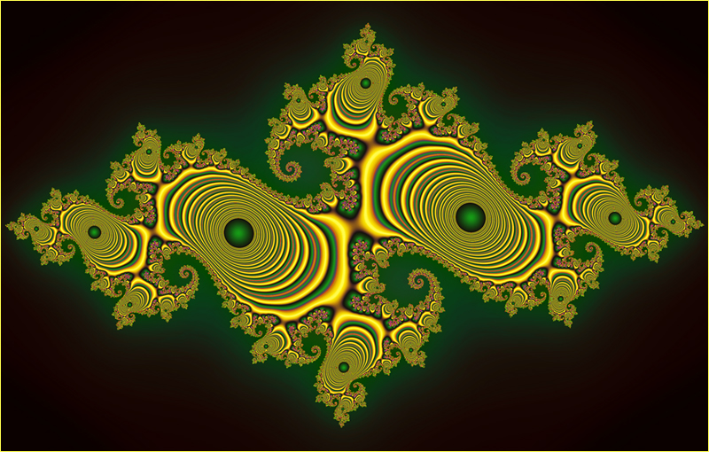
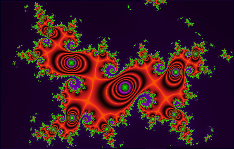
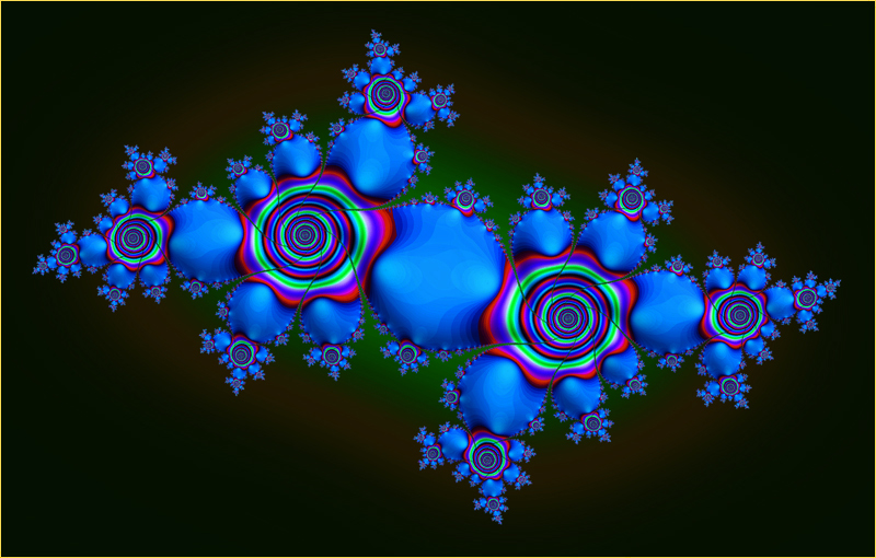
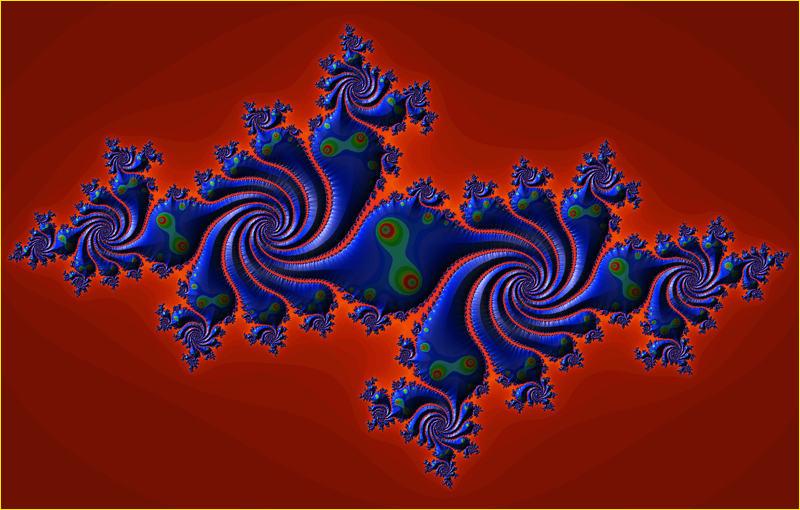
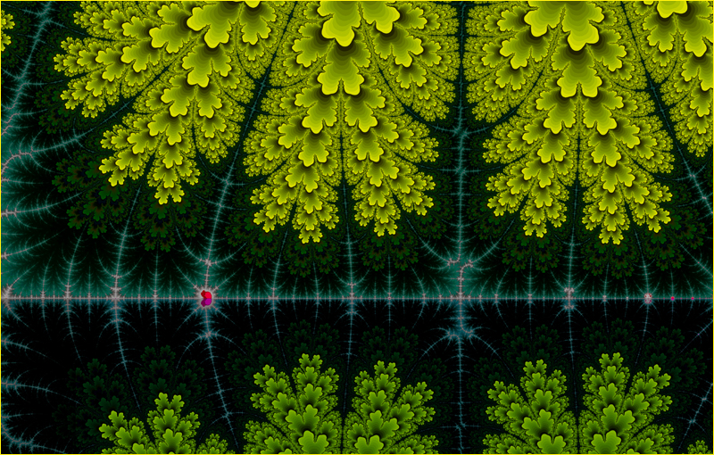
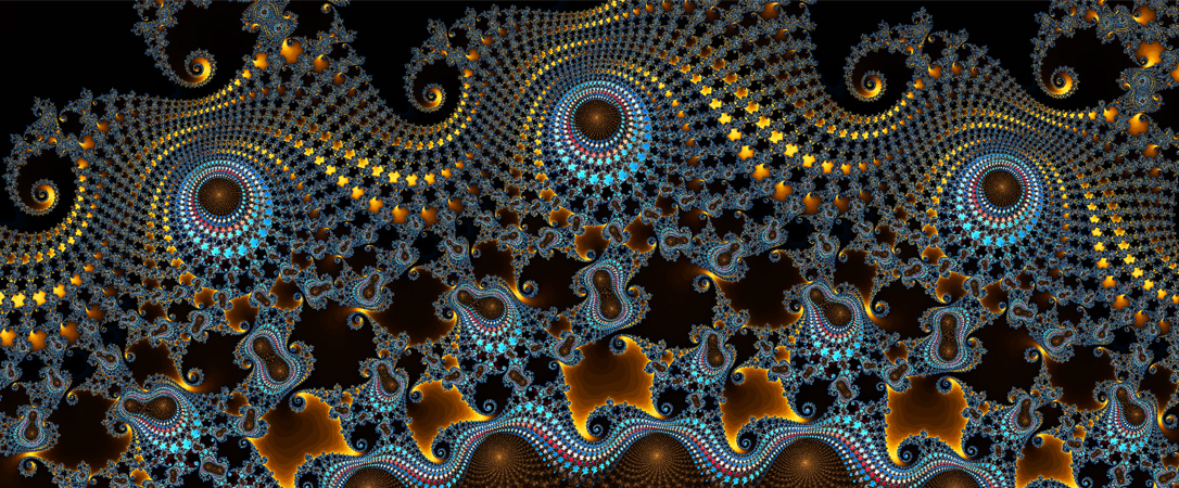
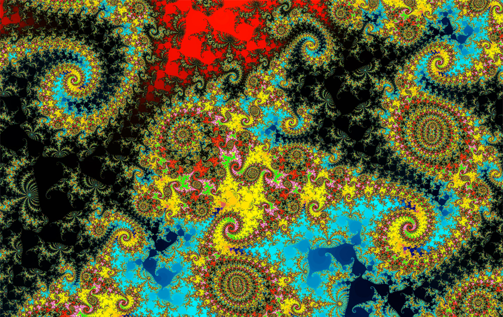
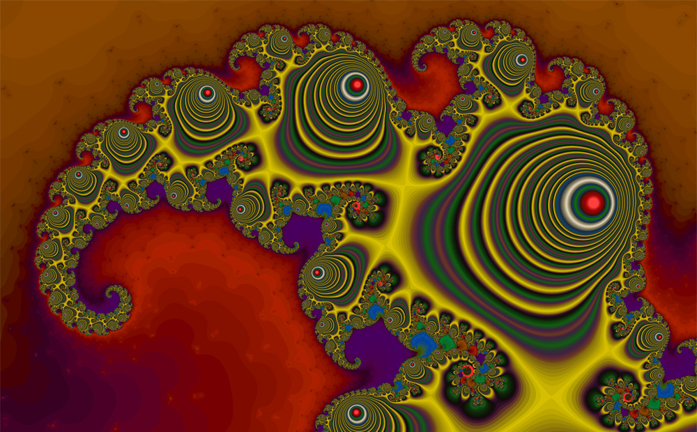
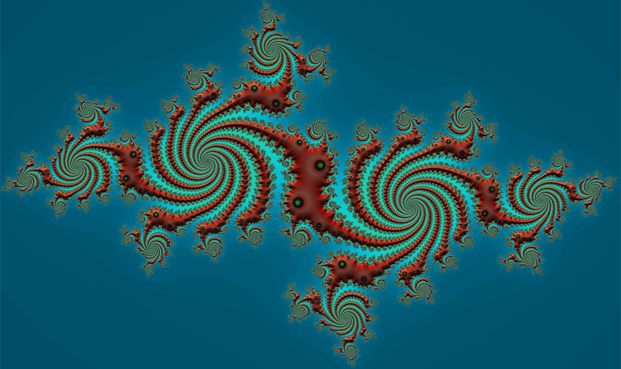
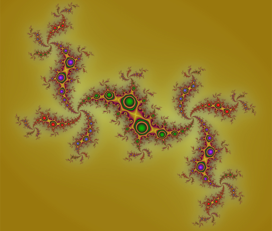
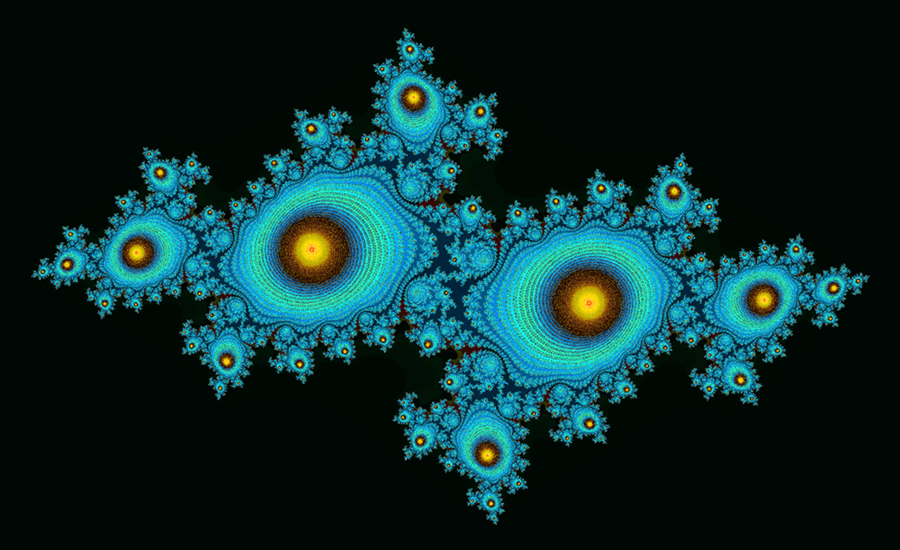
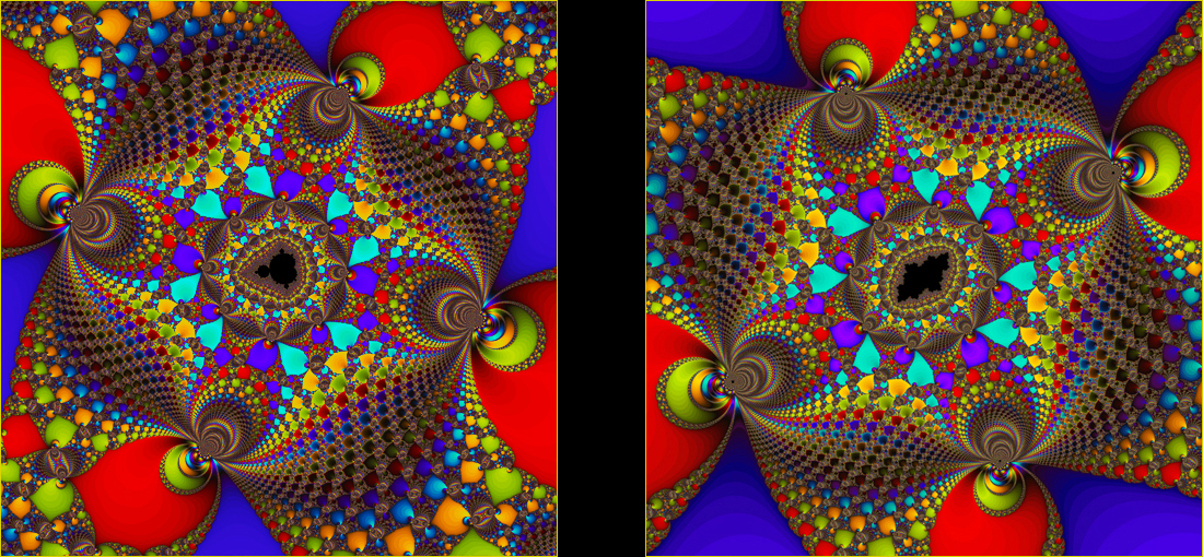
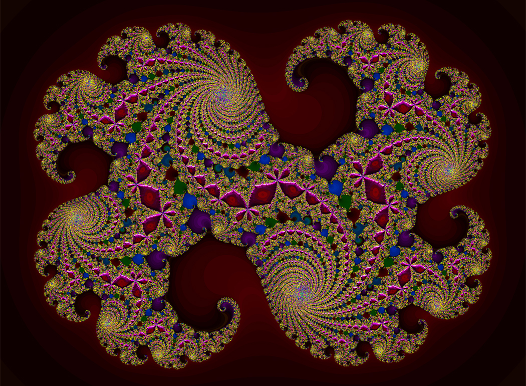
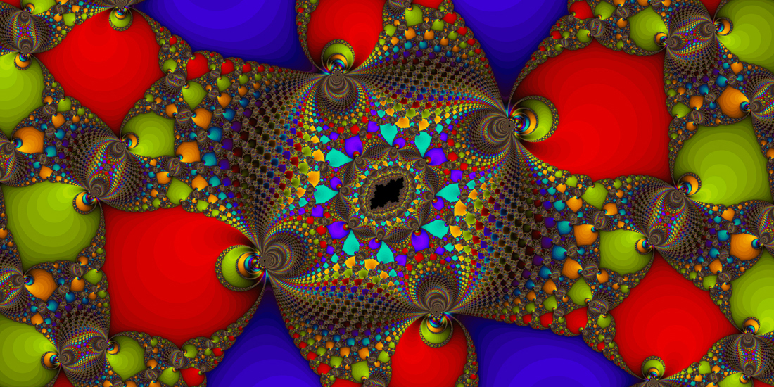
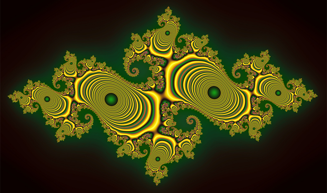
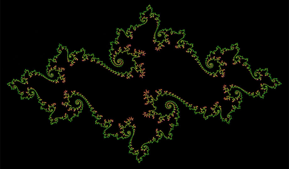
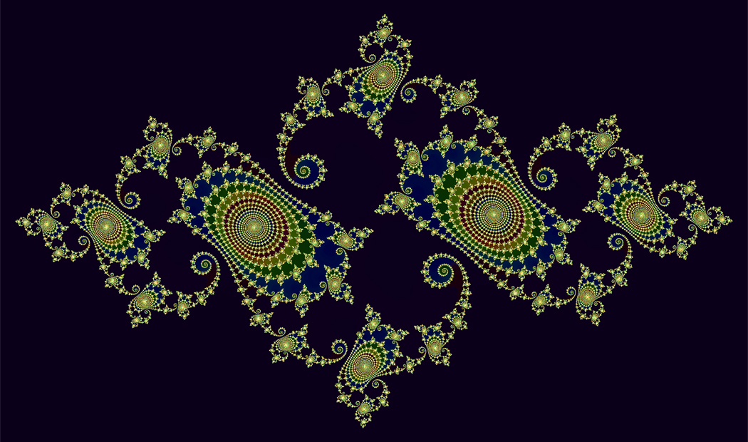
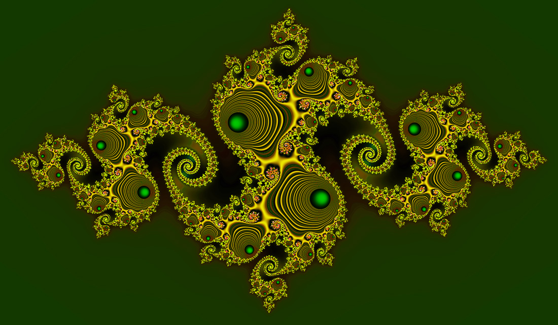
The idea of chaos quickly evolved into comprehensive chaos theory in science and at the same time its affinity with fractal art became evident. It may sound paradoxical, but the more elaborate and dazzling a fractal image, the more likely its entanglements with chaos. For example, the Julia sets became known to be chaotic and shape a great many fractal art pieces; e.g., see Figures 0.6(B), 0.6(C), 0.6(D) and 0.6(E).


Figure 0.7(A). "Autumn Leaves"


A Mandelbrot fractal from near the Area where Chaos was Discovered


Figure 0.7(B). A Mini-Mandelbrot Set


Another Mandelbrot fractal generated by the logistic equation


Figure 0.7(C). "Fractal Gems"


A Julia fractal "born" from the mini-Mandelbrot set of Figure 0.7(B); see Gallery 2D.


Googling we can find a host of
websites displaying computer-generated fractal art images, some of which are stunningly beautiful. It indicates that a large population not only appreciates the digital art form but also participates in the eye-opening creative activities. A fairly large part of this article is devoted to show how to program a computer and plot popular types of fractals generated by simple dynamical systems. It is not a text on computer programming but instead tells the general principles for fractal plotting in everyday language so as to entice more people into trying it.

Particularly exciting is the moment the fractal image generated by our personal program emerges in our computer screen, because of its potentially "astounding" artistry and built-in chaos-related unpredictability. Many of the fractal art images will stir our imaginations in the part of mathematics that is in fact quite deep and still filled with unknowns. It is plain fun.


Figure 0.8(A). "Lion's Den"


A Julia Fractal Based on a Highly Chaotic Julia Set; See Gallery 2D.


Figure 0.8(B). "Butterflies"


Go to Gallery 2D to see more examples.


Figure 0.8(C). "Snails"


Go to   Top of the Page

§ 1. Previews of § 2 - § 8
§ 3. The Mandelbrot Set
§ 6. Generalizations

Fractal Coloring Algorithms
Introduction

§ 2. The Divergence Scheme
§ 4. The Convergence Scheme
§ 7. The Logistic Equation

Gallery 2D
Prep Math


§ 5. Julia Sets
§ 8. Newton Fractals

Gallery 3D


Preparatory Mathematics

As mentioned at the outset, the text in this article is meant as an optional reading and is not needed in appreciating the fractal art images. On the other hand, people who wish to understand fractals in some depth by following the article need to know (a) elementary algebra and geometry of complex numbers and (b) beginning calculus. In addition, people interested in learning fractal plotting should have (c) some basic computer programming experience. Courses covering (a), (b) and (c) are normally available in high school.

(a) includes the practice of writing a complex number z as a point (x, y) in the xy-plane as well as the standard algebraic expression z = x + yi and ability to do basic arithmetic of complex numbers such as addition and multiplication. The complex plane means the set of all complex numbers z = (x, y) which coincides with the Cartesian xy-plane. For each complex number z = (x, y), the absolute value of z means |z| = √(x2 + y2) and it represents the distance of z from the origin O of the complex plane. More generally, if u and v are complex numbers, |u - v| represents the distance between u and v, which satisfies the triangle inequality

    |u - v| ≤ |u| + |v|.

Setting w = u - v, we get |w| ≤ |w + v| + |v|. Hence, another way of writing the triangle inequality is

    |w + v| ≥ |w| - |v|,

which will be used a few times in the upcoming sections to justify certain key propositions. The only ideas we need from (b) are the derivative and a critical point of a function where the derivative vanishes.


Figure 1.0(A).  "Dancing Seahorses"


See Fractal Coloring for the Step-by-Step Coloring Algorithm for the Image
Generated by the Mandelbrot Equation


We now introduce several preliminary ideas.

Orbits and Dynamical Systems: When we solve a mathematical problem using a computer, we frequently do it by exploiting what the machine does best, namely an iteration. It means repeating a certain process over and over, often for thousands or even millions of times, at a blinding speed. To see how it works, consider the best-known equation in fractal plotting, which we call the Mandelbrot equation for convenience:

(1.1)     zn+1 = zn2 + p ,withn = 0, 1, 2, · · · ,

where zn+1, zn and p are complex numbers and p is called a parameter. The iteration index n is especially important for fractal plotting and it is there for us to iterate the equation to generate a sequence of complex numbers once the value of p and initial value z0 are given. For instance, let p = -2 and z0 = 0. Then setting the index n = 0, 1, 2, · · · in (1.1), our properly programmed computer iterates (1.1) and calculates the sequence of numbers

   z0 = 0,  z1 = z02 + p = 02 - 2 = -2 ,z2 = z12 + p = (-2)2 - 2 = 2 ,z3 = z22 + p = 22 - 2 = 2 , · · · ,

i.e.,  z0 = 0,  z1 = -2 ,z2 = 2 ,z3 = 2 , · · · ,  z30 = 2,  z31 = 2, · · · ,

which is called the orbit of p = -2 with the initial value z0 = 0 or the orbit of z0 = 0 with the parameter value p = -2. If we hold the value of z0 at z0 = 0 and change the value of p from p = -2 to p = -1.9 in (1.1) then the computer again iterates (1.1) and quickly calculates thousands of terms in the sequence

   z0 = 0,  z1 = -1.9,  z2 = 1.71,  z3 = 1.0241, · · · ,  z30 = -1.1626,  z31 = -0.5483, · · · ,

which is now called the orbit of p = -1.9 with the initial value z0 = 0 as well as the orbit of z0 = 0 with the parameter value p = -1.9. It is important to note that an orbit may change its behavior drastically if the parameter value p changes slightly. For instance, unlike the orbit of p = -2 which becomes static after time n = 2, the orbit of p = -1.9 keeps moving along the real axis of the complex plane in a seemingly unpredictable way as time n progresses. Note that we refer to the index n as time or instant.


Figure 1.0(B). "Turquoise Lion"


Technical Description: The Julia Set of p = (0.281215625, 0.0113825)
On a z-Canvas Centered at z0 = (0, 0)
Generated by the Mandelbrot Equation


Figure 1.0(C).  "Esmeralda Lion"


Technical Description: The Julia Set of p = (0.281150625, 0.011546875)
On a z-Canvas Centered at z0 = (0, 0)
Generated by the Mandelbrot Equation


We have used only real numbers for simplicity, but the orbits used in fractal plotting are sequences of complex numbers in the complex plane. Because most of the orbits dance around in the complex plane with time n, it is appropriate to call a collection of orbits a dynamic mathematical system or dynamical system. For example, the Mandelbrot equation (1.1) is a dynamical system consisting of infinitely many orbits of complex numbers, one orbit zn for each choice of values of p and z0. As we shall see, there are infinitely many dynamical systems including the Mandelbrot equation (1.1) and the logistic equation (7.1), each of which generates infinitely many fractals.


Figure 1.1(A). "Circus Seahorses"


Technical Description: The Julia Set of p = (0.03697296, 0.55091235)
On a z-Canvas Centered at z0 = (0, 0)
Generated by the Dynamical System zn+1 = zn3 + zn + p


Figure 1.1(B).  "Circus Elephants"


Technical Description: The Julia Set of p = (0.0641826, 0.5406694)
On a z-Canvas Centered at z0 = (0, 0)
Generated by the Dynamical System zn+1 = zn3 + zn + p


Canvases: We begin with a simple example. 
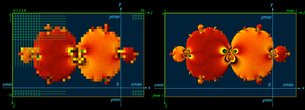
Let R be the rectangle in the
complex plane defined by -2 ≤ x ≤ 2 and -1.28 ≤ y ≤ 1.28 and suppose we wish to plot the graph of the inequality x2 + y2 ≤ 1 on R using a computer. We first decompose R into, say, 50 × 32 miniature rectangles of equal size called picture elements or pixels and then represent the pixels by pixel coordinates (i, j) in such a way that the upper left and lower right pixels are (0, 0) and (49, 31), respectively. Thus, the i- and j-axes of the pixel coordinate system are the rays emanating from the upper left corner of R and pointing east and south, respectively; see the diagram in Figure 1.2(A) on the left.

Let imax = 50, jmax = 32, xmin = -2, xmax = 2, ymin = -1.28 and ymax = 1.28. Then for each i = 0, 1, 2, · · ·, imax-1 and j = 0, 1, 2, · · ·, jmax-1, the pixel (i, j), which is a rectangle, contains infinitely many complex numbers (x, y). For our computational purpose, we choose exactly one representative complex number (x, y) in the pixel (i, j) by setting

(1.2)    Δx = (xmax - xmin) / imax; Δy = (ymax - ymin) / jmax,

(1.3)    x = xmin + i Δx;  y = ymax - j Δy.

Consequently, we may view R as the rectangle comprising imax × jmax = 50 × 32 pixels, each of which has a unique representative complex number. The rectangle R with the pixel structure is called a canvas for plotting the output image with the image resolution of 50 × 32 pixels.

Plotting the graph of the inequality x2 + y2 ≤ 1 on the canvas is now easy. For each pixel (i, j), we examine its representative complex number (x, y) on the canvas R. If it satisfies the inequality, color the pixel red, and otherwise, color it white. Since the coloring process uses only finitely many pixels of the canvas R, the output image that resembles the Japanese flag is an approximation of the true graph. The greater the number of pixels, the higher the image resolution and the more accurate the output image.

Figure 1.2(A) shows two approximations of a fractal called "Goldfish in Love." The one on the left is painted on a canvas with 50 × 32 pixels and the other on a canvas with 500 × 320 pixels.


Figure 1.2(A). "Goldfish in Love" with Different Image Resolutions


Technically, a canvas can be defined by any positive integers imax and jmax and any real numbers xmin, xmax, ymin and ymax with  xmin < xmax and ymin < ymax, but we normally impose the ratio equality

(1.4)    (ymax - ymin)/(xmax - xmin) = jmax/imax

on the input values xmin, xmax, ymin and ymax. Then (1.4) implies that Δx = Δy in (1.2) so each pixel is a square as shown in Figure 1.2(A). This way the red circle in the aforementioned output would not look oval.


Figure 1.2(B). "Jellyfish Queue"


Technical Description: A Local Image of the Mandelbrot Set on a p-Canvas
Centered at p = (0.28212284496875, 0.0110092373125)
Generated by the Mandelbrot Equation with z0 = 0


Figure 1.2(C). Mini-Mandelbrot Sets


Technical Description: A Mandelbrot Fractal of z0 = i/√3 on a p-Canvas
Centered at p = (0.00401324, -1.98544205)
Generated by the Dynamical System zn+1 = zn3 + zn + p


p-Canvases and z-Canvases:  Consider any
dynamical system like the Mandelbrot equation (1.1) comprising infinitely many orbits zn of complex numbers, one for each choice of values of z0 and p, both varying through the complex plane. Recall that a canvas is a rectangle R in the complex plane consisting of pixels (i, j), each of which has a representative complex number (x, y). In fractal plotting, we view the complex numbers representing the pixels as values of p and call the canvas R a p-canvas or view these complex numbers as values of z0 and call the canvas R a z-canvas.

Plotting a fractal on a p-canvas is, roughly speaking, as follows: Choose a value of z0, say z0 = 0, and an appropriate p-canvas following the direction in
§ 2 or § 4. For each pixel (i, j) on the p-canvas R, use its representative parameter p and the dynamical system to generate the orbit of p with the initial value z0 = 0. We then use a certain property of the orbit to color the pixel (i, j). As we have seen, the orbits from adjacent pixels on the p-canvas may have drastically different behaviors, possibly causing dramatic color changes in the image painted on the p-canvas.

Plotting a fractal on a z-Canvas is similar except that here we use orbits of z0 (with a fixed parameter value p) corresponding to all z0 on the z-canvas instead of orbits of varying p with a fixed initial value z0. We call a fractal plotted on a z-canvas a Julia fractal, as it is typically a colorful fractal art image depicting a Julia set; see Figure 0.6(B). Because Julia sets are colorless subsets of the complex plane belonging to fractal geometry, there is a clear difference between a Julia set and a Julia fractal, but after a while, we'll follow the common practice of identifying them and calling the colorful version a Julia set rather than a Julia fractal.

For the similar reason, a fractal plotted on a p-canvas is called a Mandelbrot fractal. It is normally an artistic view of the Mandelbrot set, but again, we will call the colorful version the Mandelbrot set rather than a Mandelbrot fractal. There are some exceptional cases, however, like when we discuss a "Mandelbrot-like" set generated by a dynamical system other than the Mandelbrot equation. In such a case, the image on the p-canvas will be called a Mandelbrot fractal instead of the Mandelbrot set.


Figure 1.2(D). "Jady Unicorns"


Technical Description: A Julia Fractal of p = (-0.3959, 0.0312)
On a z-Canvas Centered at z0 = (-1.254375, 0.052756)
Generated by the Dynamical System zn+1 = zn4 + zn + p


Figure 1.2(E). "Metallic Unicorns"


Technical Description: A Julia Fractal of p = (-0.39985, 0.02025)
On a z-Canvas Centered at z0 = (-1.254375, 0.052756)
Generated by the Dynamical System zn+1 = zn4 + zn + p


Figure 1.2(F). "Gold Elephants"


A Subset of the Julia Set in Figure 1.7(D) Painted on a z-Canvas


Figure 1.2(G). "Running Corolla"


Technical Description: The Julia Set of p = (-1.1128, 0.23076)
On a z-Canvas Centered at z0 = (0, 0)
Generated by the Mandelbrot Equation


Geometric Similarity:  We say that two objects in a plane are geometrically similar if one can be obtained from the other by uniform scaling (enlarging or reducing), translation, rotation and/or reflection; see
Wikipedia for detail. Geometrically similar objects are said to be congruent if one can be obtained from the other without uniform scaling. We learn the concept of geometric congruence in high school geometry mostly using triangles and conditions like "side-angle-side." In this article, we don't distinguish geometrically similar fractals and treat the images such as the ones shown below to be identical.


Technical Description: See Figure 6.0 in § 6


In geometry, we generally imagine that objects such as triangles are made of a rigid material like a metal plate. If they are made of something totally elastic like pizza dough that can be deformed by kneading then we are in the realm of topology instead of geometry. Here are some of the basic topological ideas that will appear in the upcoming sections.

Topological Ideas:  We say that nonempty sets A and B of points in the complex plane are topologically equivalent if there is a continuous function h mapping A onto B in a one-to-one fashion such that its inverse h-1 is also continuous. Such a function h is called a homeomorphism, which is a formal notion of "kneading a pizza dough to change its shape from A to B." For example, a triangle and a square are topologically equivalent or homeomorphic while they are not geometrically similar.


Technical Description: See Example 5 in § 5


A topological property means a property of a set that is preserved under a homeomorphism. For example, being connected as "one piece" is a topological property because if A and B are homeomorphic and A is connected then B must be connected as well. Similarly, having no holes is a topological property. "Tearing" or "poking a hole" on a pizza dough is not part of "kneading." In § 3, we will define connectedness more carefully as it plays an important role in fractal geometry.

To see a few more topological ideas which we will encounter later on, consider a circle in the complex plane. The disk that comprises all of the points inside the circle but none of the points on the circle is called an open disk. Let A be a set of points in the complex plane and call the set of points not in A the complement of A. Then a point b is called a boundary point of A if every open disk about b contains a point belonging to A and a point belonging to the complement of A. The set of all boundary points of A is called the boundary of A and the largest subset of A without any of its boundary points is called the interior of A.

We say that A is closed if it contains all of its boundary points, and A is open if it contains none of its boundary points. Thus, closed and open sets are generalizations of closed and open intervals on the real number line. We also say that A is bounded if there is a circle in the complex plane that encloses A, and A is compact if A is closed and bounded. Compactness, closedness and openness are all topological properties but boundedness is not.


Figure 1.4(B).  The Mandelbrot Set
With its Complement (Left Green), Boundary (Left Amber) and Interior (Right)


Plotted on a p-Canvas
by the Divergence Scheme of § 2
Plotted on a p-Canvas
by the Convergence Scheme of § 4


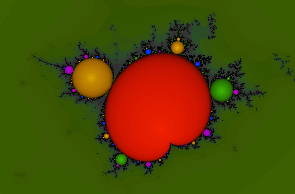
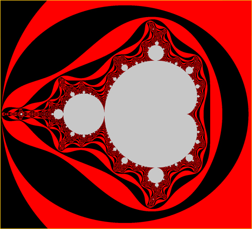
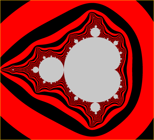
As we'll see, the Mandelbrot set generated by the
Mandelbrot equation is bounded so its global figure fits in a circle or a rectangle like in Figure 1.4(B), and from the shape of its black silhouette, it is often nicknamed "Warty Snowman" lying sideways. A part of the global image is called a local image, but a local image in fractal art is usually given by zooming in on a microcroscopic rectangular neighborhood of a point that is very near or on the border of the snowman's silhouette.

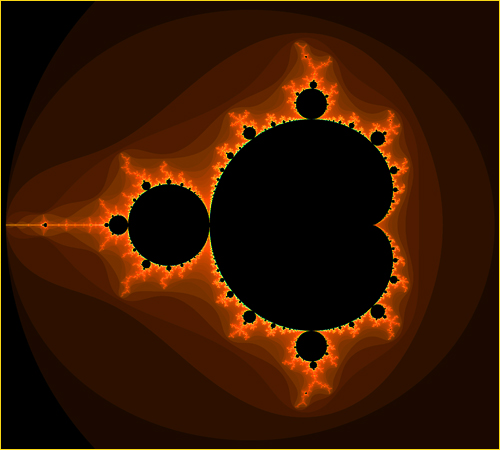
Because the Mandelbrot set is also known to be closed, its boundary, which coincides with the snowman's silhouette's border, is a part of the Mandelbrot set. It is also known that the boundary has the "topological dimension" of 1, meaning intuitively that it comprises razor thin "filaments" without thickness, just like the boundary of a circular disk. So, the boundary is mostly invisible in local images unless we "light up" their filaments like in a tungsten light bulb; see Figure 1.4(C) shown below.

As Figure 1.4(B) shows, the filaments are like branched hairs growing outwards from the warty snowman and known to carry infinitely many miniature copies of the snowman, which we call "mini-Mandelbrot sets." One of them is visible in Figure 1.4(C) and, yes, the boundary of the Mandelbrot set is incredibly intricate.


Figure 1.4(C).  A Local Image of the Mandelbrot Set
With its Complex Boundary Highlighted by the Goldish Color


Painted on p-Canvases Centered at p = (0.281229249, 0.011344208)
See "Daytime View" and "Nighttime View" of a Fractal in § 3


Go to   Top of the Page

§ 1. Previews of § 2 - § 8
§ 3. The Mandelbrot Set
§ 6. Generalizations

Fractal Coloring Algorithms
Introduction

§ 2. The Divergence Scheme
§ 4. The Convergence Scheme
§ 7. The Logistic Equation

Gallery 2D
Prep Math


§ 5. Julia Sets
§ 8. Newton Fractals

Gallery 3D


§ 1.  Previews of Upcoming Sections § 2 ― § 8

In 2008, PBS broadcast a NOVA program proclaiming that the Mandelbrot set had become "the most famous object in modern mathematics." Naturally then, we begin our stories with the Mandelbrot set and devote a large part of the article to a myriad of its attributes that fascinate mathematicians and artists alike. The Mandelbrot set popularized the fractal plotting by computers and has been the gold standard for all types of fractals.

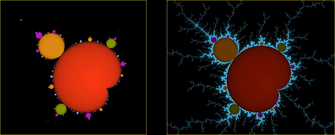
In
§ 2, we state the notion of an orbit that diverges to ∞ and define the Mandelbrot set, denoted by , using the Mandelbrot equation (2.1) and its critical point. In § 4 we also introduce the notion of an orbit that converges to a cycle of period k for some positive integer k and in conjunction with § 2 explain how to plot ℳ globally and locally on p-canvases using algorithms called the divergence and convergence schemes. Figure 1.4(B) shows global images of ℳ contrasting the two distinct algorithms, while Figure 1.4(C) shows a local image of ℳ together with its complex boundary. As we have seen, ℳ contains its boundary as its subset.


Figure 1.5(A). A Local Image of the Mandelbrot Set ℳ


This is a local image of Figure 2.3 plotted by the divergence scheme.


By far the biggest attraction of ℳ is the fact that it conceals a greater number of varying local images than the number of stars in the universe, together with the simplicity of the divergence scheme (aka the "escape time algorithm") that allows even amateurs to find many of them and turn them into beautiful art pieces. Thus, its appeals have extended way beyond mathematical communities, contributing ℳ to gain its monumental popularity―which is unheard of for an object in mathematics.

In
§ 3, we discuss some of the important mathematical properties of ℳ, focusing on its boundary. Note that in Figure 1.4(C) the goldish boundary comprising razor thin filaments gets increasingly more intricate and space-filling as it gets nearer the mini-Mandelbrot set until it gets an appearance of being solidly painted. It makes the painted area look two-dimensional. Shishikura's theorem formally explains a phenomenon like that in terms of "fractal dimensions," and shows, in effect, that no figures in the plane are more complex than the boundary of ℳ. It boosts the Mandelbrot set ℳ to be one of the most complex figures ever plotted on a plane.


Figure 1.5(B).  Periodicity Diagram of ℳ


We call λ the period of a mini-Mandelbrot set


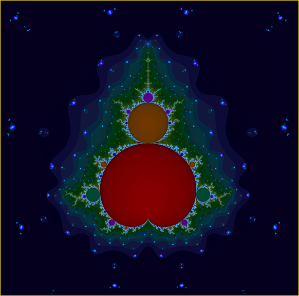
In
§ 4, we turn our attention to the interior of ℳ and use Mandelbrot's idea as a cue to define an atom to be a connected component of the interior. Then atoms include all of the disks and cardioids visible in ℳ, and as per the "density of hyperbolicity" conjecture, all atoms are associated with periods of certain cycles. A part of the association between atoms and periods is illustrated by the meticulously aligned numerical structure shown above in the periodicity diagram.

In spite of all these astounding complexities of ℳ, Adrien Douady and John H. Hubbard established earlier that ℳ is topologically tidy as it is compact, connected in one piece and without holes. The connectedness of ℳ is particularly important and called the Douady-Hubbard Theorem. The next-step problems of whether ℳ is pathwise connected and whether ℳ is locally connected are conjectured affirmatively but still remain unsolved, despite the efforts by some of the world's brightest minds.

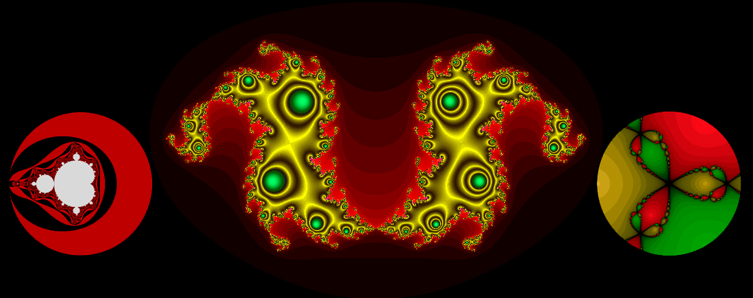
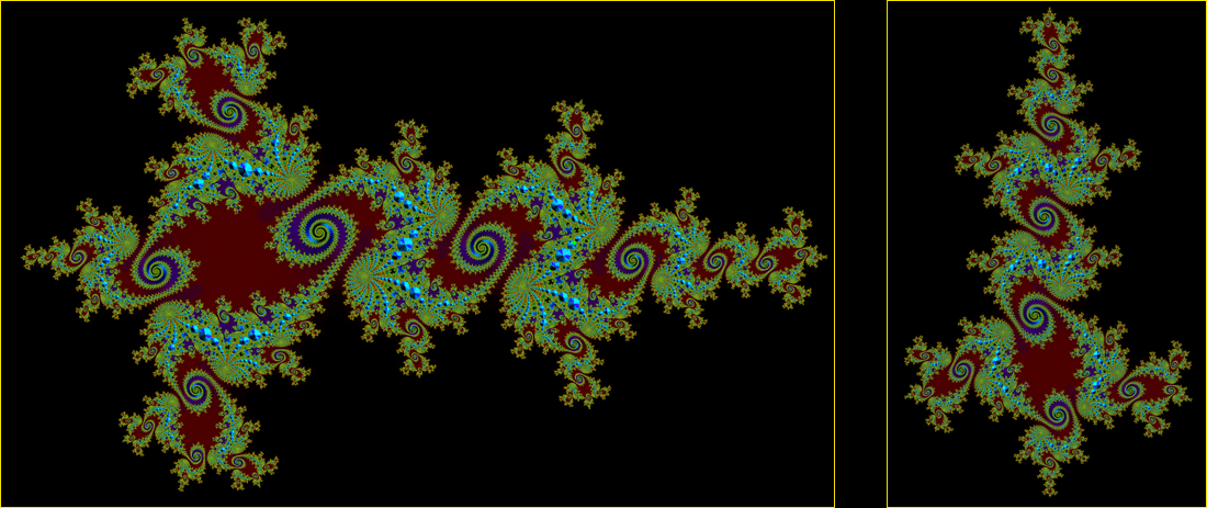
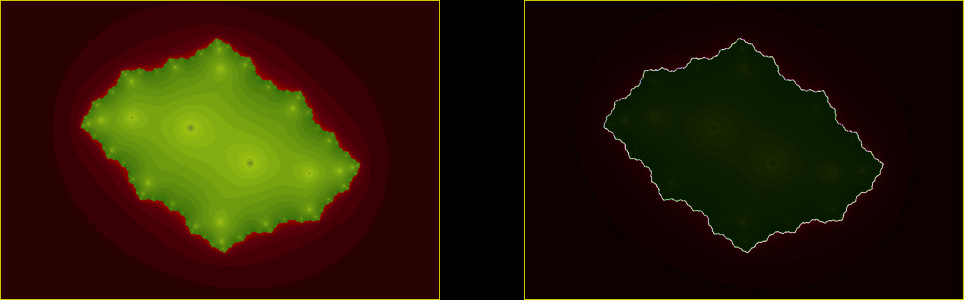
In § 5, we define, given a parameter p in the complex plane, the filled-in Julia set of p generated by the Mandelbrot equation and show how to plot it on a z-canvas using the divergence and possibly convergence schemes. If p belongs to an atom of ℳ, then the period of the atom affects the shape of the filled-in Julia set in an amazing and sometimes amusing way, although the exact cause is shrouded in mystery. It makes the periodicity diagram all the more important in plotting filled-in Julia sets. For example, the image shown below is the filled-in Julia set of a parameter chosen from an atom of period 9 (near the "neck of the warty snowman"), while Figure 1.4(A) shows two filled-in Julia sets born from the same atom of period 17 × 5 (which is near the cusp of the cardioid).


Figure 1.6(A). "Hydra of Lerna" Born from an Atom of Period 9


Technical Description: The Filled-in Julia Set of p = (-0.661, 0.3434)
On a z-Canvas Centered at z0 = (0, 0)
Generated by the Mandelbrot Equation


Figure 1.6(B). "Dancing Beans" Born from an Atom of What Period?


Technical Description: The Filled-In Julia Set of p = (0.262, 0.5701)
On a z-Canvas Centered at z0 = (0, 0)
Generated by the Mandelbrot Equation


The boundary of a filled-in Julia set is called a Julia set. The Julia sets are known to be
chaotic and their shapes play a key role in many of the fractal art images; see Figure 0.6(B). The most consequential theorem on the Julia sets is a corollary to the Fatou-Julia Theorem, called the fundamental dichotomy, as it motivated the birth of the Mandelbrot set. It states that the Julia set of any parameter p is either connected or totally disconnected, dividing up the complex plane comprising the parameters into two parts. Mandelbrot wanted to use a computer and visualize the dichotomy, so he initially defined:

(†)  The set ℳ (later named the "Mandelbrot set") means the set of all parameters in the complex plane whose Julia sets are connected.

The Fatou-Julia theorem also implies that the Julia set of p is connected if and only if the
critical orbit of p does not diverge to ∞. Thus, Mandelbrot knew that (†) is equivalent to the computer-friendly definition of § 2, providing the easy algorithm to compute ℳ. This also explains why the critical point plays a crucial role in the Mandelbrot set.


Figure 1.6(C). "Hydra's Ash"


Technical Description: The Julia Set of p = (-0.6891, 0.27896)
which is near an atom of period 11 but outside of ℳ


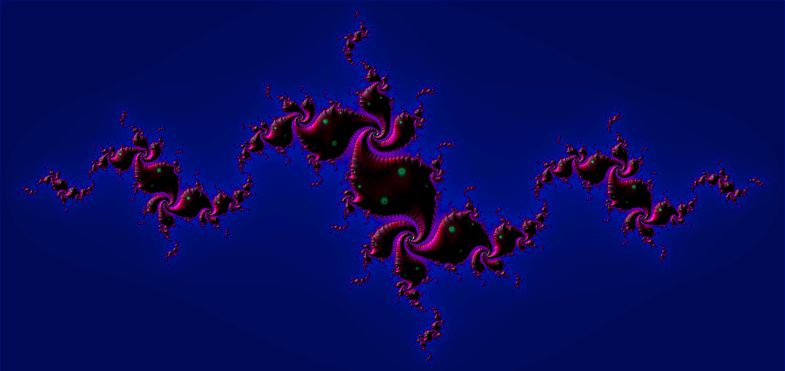
Note that the Julia set of
Figure 1.6(B) is connected as its parameter belongs to ℳ. but the Julia set of Figure 1.6(C) shown above is totally disconnected. It is interesting and important to note in the latter that the period of the nearby atom, namely k = 11, still shows in the shape of the Julia set as the number of the "hydra's heads."

To further consolidate the close-knit relations between ℳ and the Julia sets given by (†), we will also discuss Tan Lei's Theorem in § 5, which explains why we frequently observe striking similarities in appearance between local images of ℳ and Julia sets. The phenomenon is so prevalent that the Mandelbrot set ℳ is often called an "index" to all Julia sets.


Figure 1.6(D). Local Similarity
Between the Mandelbrot Set (left) and a Julia Set


For details, see Local Similarities between ℳ and Julia Sets


As we have just noted, the Mandelbrot set is uniquely determined by the
critical point z0 = 0 of the Mandelbrot equation. So, what happens if we deal with a dynamical system with multiple critical points?

In § 6, we extend the Mandelbrot equation to more general dynamical systems, and, in particular, consider the relatively simple cubic dynamical system (6.2) with two critical points z0 = ± i / √3 = ± (0, 1 / √3).

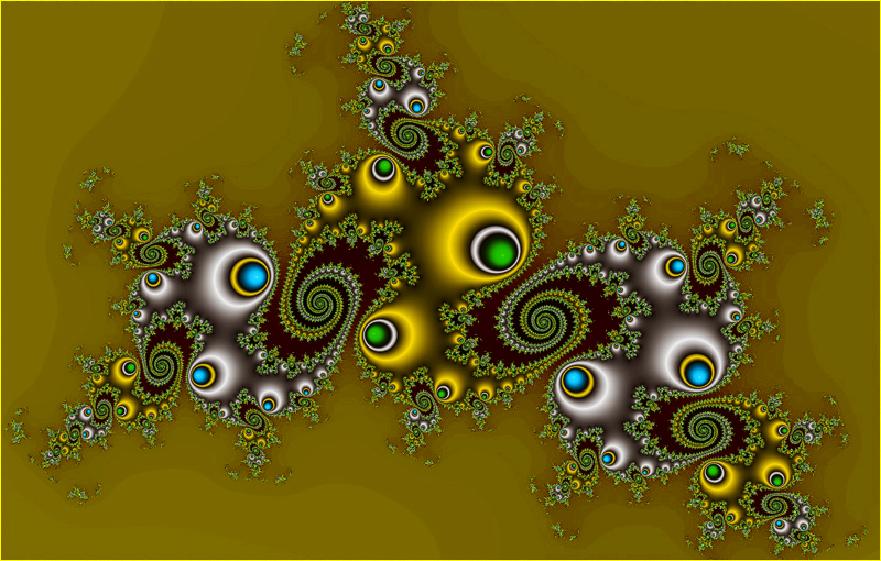
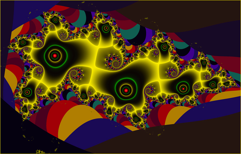
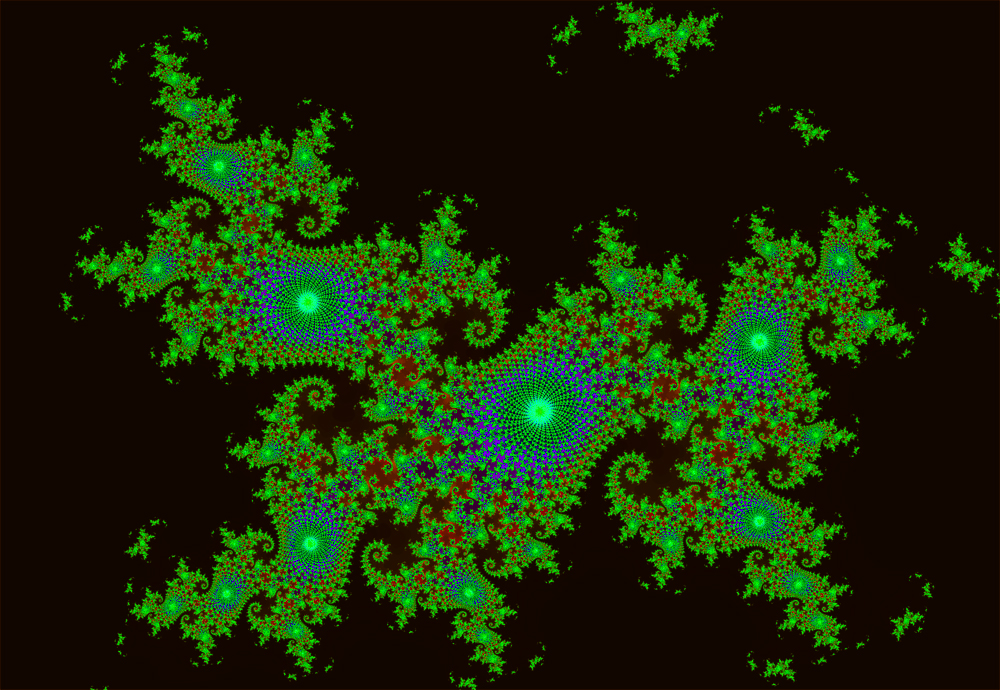
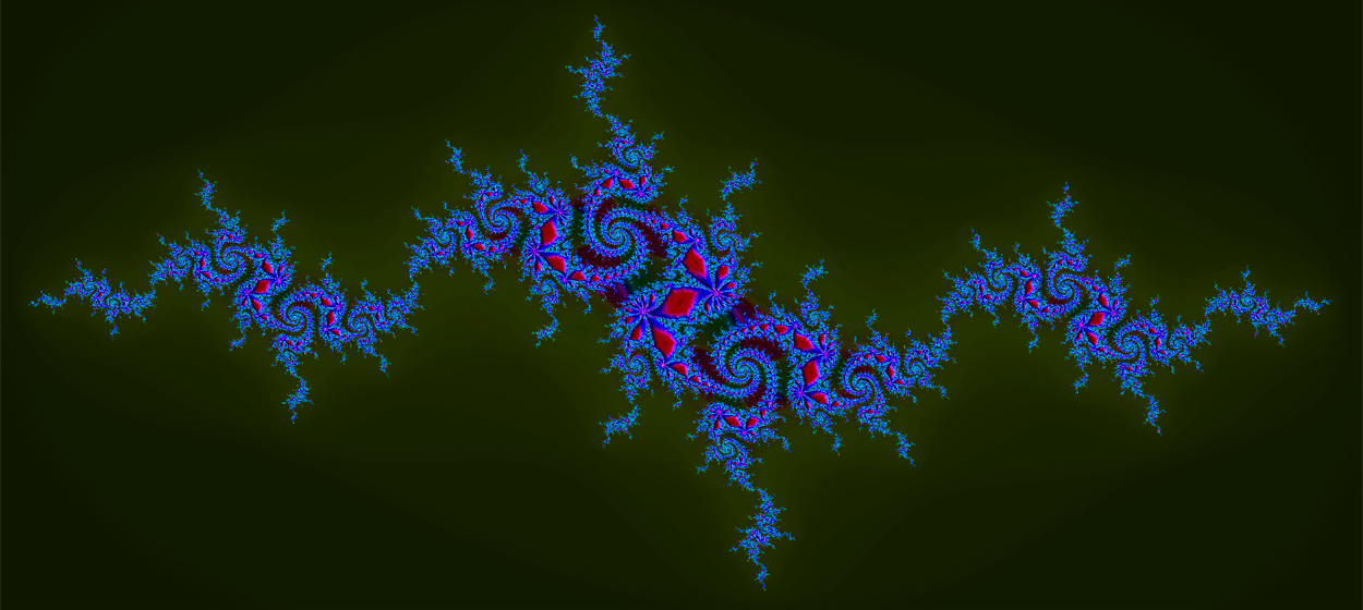
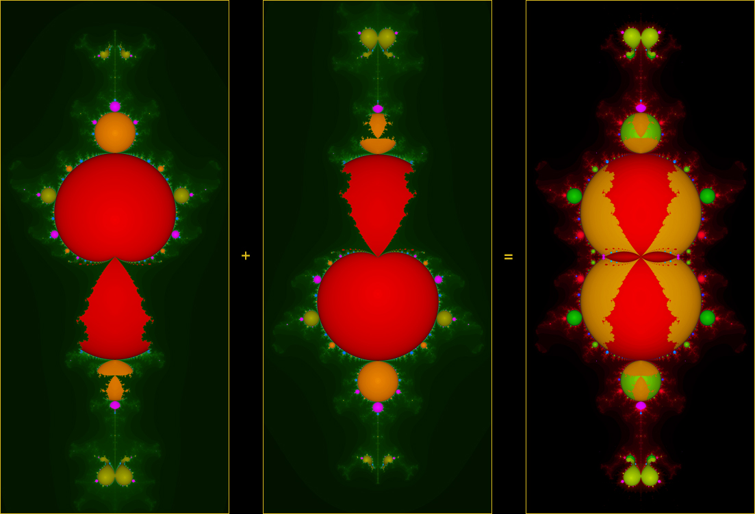
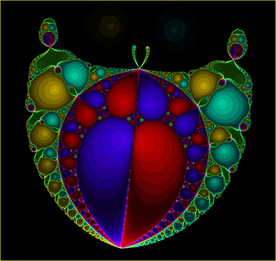
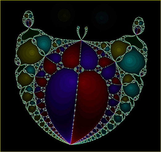
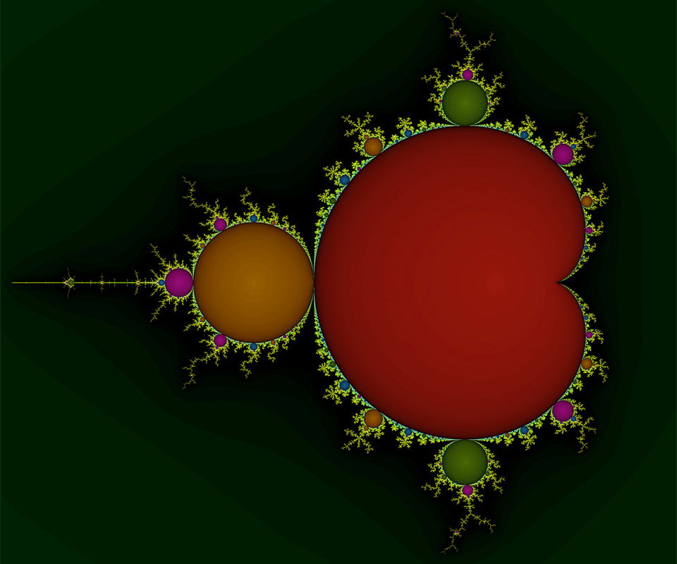
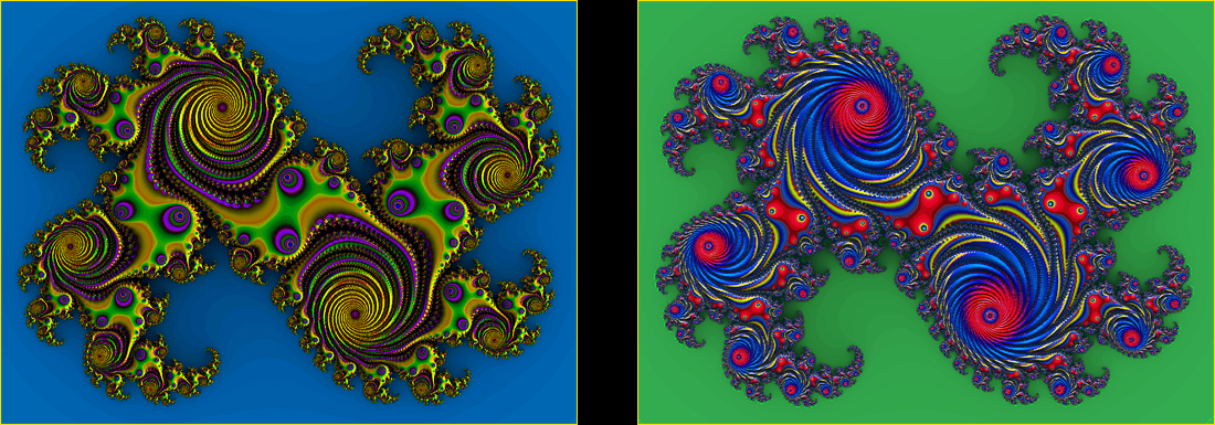
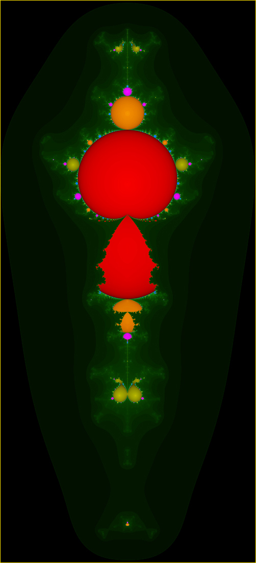
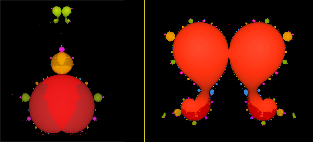
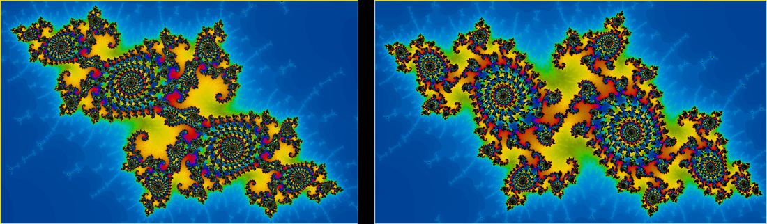
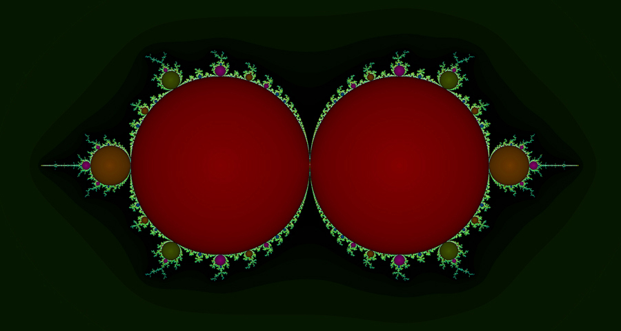
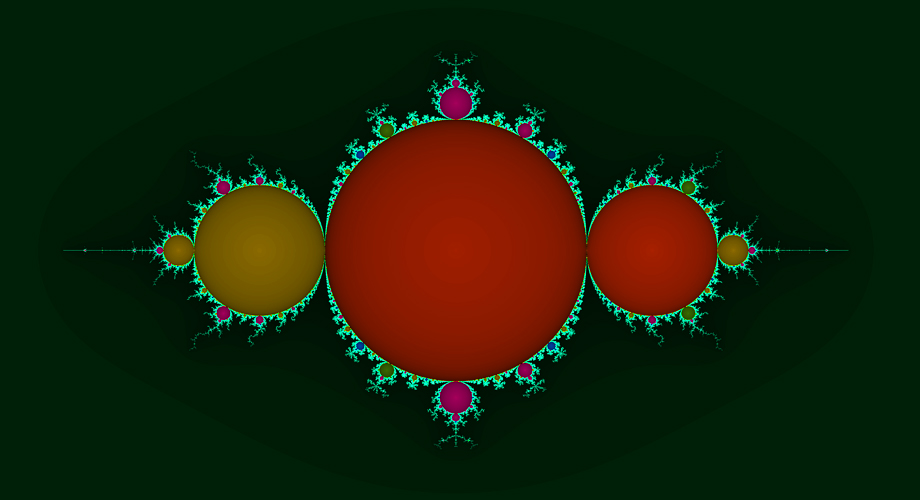
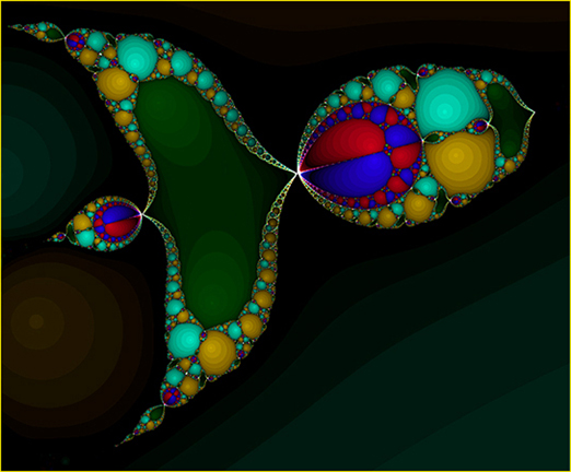
If we define and generate the "Mandelbrot sets" using (6.2) and the two critical points, we get rather comical fractals called the Speared Mandelbrot Sets1 and ℳ2; see Figure 1.7(A). To be precise, ℳ1, for instance, corresponds to z0 = i / √3 and is the portion not including the dark green background. It does include, however, the mini-Mandelbrot set seen near the bottom of Figure 6.1 like an isolated island, but it is omitted from Figure 1.7(A) for simplicity. The tip of the "spearhead" turned out to be the origin (0, 0) of the complex plane and ℳ2 is the mirror image of ℳ1 through the real axis of the complex plane.

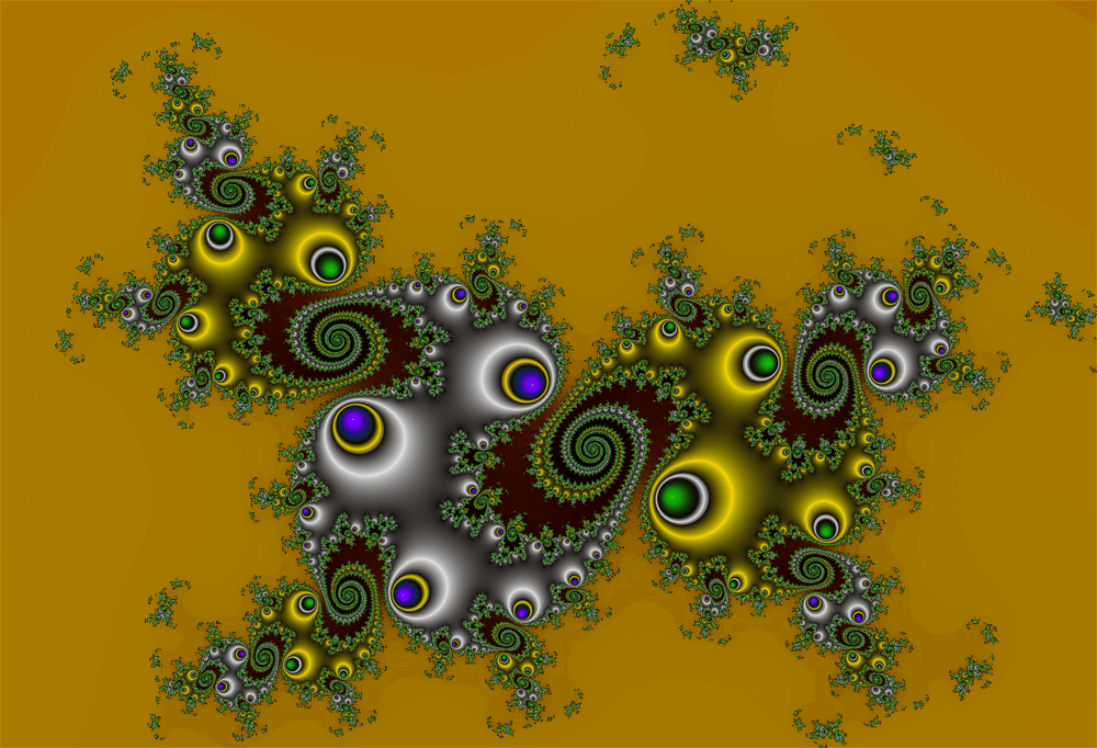
Atoms of ℳ1, for instance, are again defined to be connected components of the interior of ℳ1 and are in a wide variety of shapes that include the interior of a blue disk as well as the interior of the red spearhead.


Figure 1.7(A). "Atomic Fusion" (Right)
Of the Speared Mandelbrot Sets (Left and Center)


1

2

1 ∪ ℳ2


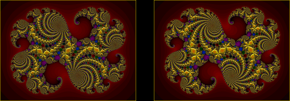
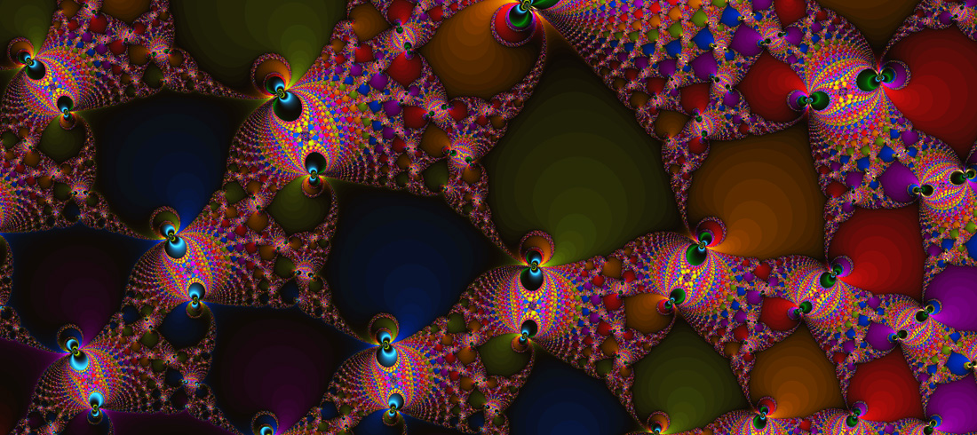
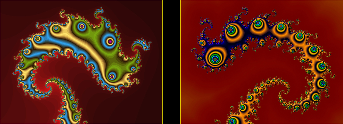
In addition to numerous local images such as
Figure 1.2(C) that are similar to those from the Mandelbrot set, ℳ1 and ℳ2 have numerous others including Figure 1.7(B) and the first image of Figure 1.7(C) shown below, where some of the atoms appear to break into fragments. Interestingly, all of the fragments disappear in the third image of Figure 1.7(A), which we call "Atomic Fusion," given by superimposing ℳ1 and ℳ2.


Figure 1.7(B). "Burst Mandelbrot Set"


See the bottom of ℳ2 in Figure 1.7(A)


Figure 1.7(C). "Atomic Fusion" (Right) of the Burst Mandelbrot Set (Above)


See the bottom of ℳ1 in Figure 1.7(A) See the bottom of ℳ1 ∪ ℳ2 in Figure 1.7(A)
Note: Colors don't match in Figures 1.7(A)(B)(C)


As we will see in
§ 6, "Atomic Fusion" has a handy application in the pictorial interpretation of the Fatou-Julia Theorem and the classification of the Julia sets given by the dynamical system (6.2). There we learn that the Julia set of a parameter p is connected if p belongs to 1 ∩ ℳ2 and it is totally disconnected if p belongs to the complement of 1 ∪ ℳ2. Thus, if the Julia set of a parameter p defies the dichotomy, then p belongs to the "symmetric difference"

   1 Δ ℳ2 = (1 ∪ ℳ2) - (1 ∩ ℳ2).

Computer experiments show that the converse of the last statement seems to hold but it is not known for sure. Here are examples:


Figure 1.7(D). "Flying Lion"


Technical Description: The Julia Set of p = (0.00033, -2.0006785)
On a z-Canvas Centered at z0 = (0, 0) Generated by (1.5)
The Julia set is disconnected but not totally disconnected.


Figure 1.7(E). "Seahorse Family"


Subset of the Julia Set in Figure 1.1(A)
The Julia set is disconnected but not totally disconnected.


Figure 1.7(F).  "Gold Dragon"

Technical Description: The Julia Set of p = (0.0618974, 0.5400784)
On a z-Canvas Centered at z0 = (0, 0) Generated by (1.5)
The Julia set is connected.


Figure 1.7(G).  "Pearly Dragon"
Technical Description: The Julia Set of p = (0.0352236, 0.5448064)
On a z-Canvas Centered at z0 = (0, 0) Generated by (1.5)
The Julia set is totally disconnected.


Finally, here are a couple of examples by a cubic dynamical system other than
(1.5):


Figure 1.7(H). "Dancing Metabo Seahorses"


Technical Description: The Julia Set of p = (-1.022, 0.14846)
On a z-Canvas Centered at z0 = (0, 0)
Generated by the Dynamical System zn+1 = zn(zn2 + p)


Figure 1.7(J). "Cloisonné Turtle"


Technical Description: Subset of the Julia Set of p = (-1.0158, 0.1449)
On a z-Canvas Centered at z0 = (0, 0)
Generated by the Dynamical System zn+1 = zn(zn2 + p)


In
§ 7, we go back to the Mandelbrot set ℳ and discuss possibly the most charming feature it possesses, which is the striking simplicity of the Mandelbrot equation (1.1) generating all the wonders of ℳ we have witnessed. Does it come at a cost? The answer turned out to be "no" in the sense that the "Mandelbrot set" ℳ ' defined by any quadratic dynamical system and (†) is essentially the same as ℳ.

Rather than showing this fact in full generality (which can be done by high school algebra), we will verify it using a special quadratic dynamical system called the logistic equation. The process involves the important idea of the "conjugacy" between two dynamical systems. As mentioned in Introduction, the logistic equation became famous with the advent of chaos and is interesting in its own right.

We will also show several examples of fractals from the logistic equation, even though similar fractals can be found by the Mandelbrot equation theoretically. Art involves more factors than mathematics such as colors and textures, etc. making it impossible to reproduce exactly the same images by any means. In art, we can also deviate from standard procedues such as using critical points and conduct computer experiments. Here's an example:


Figure 1.8(A). "Pearly Elephants"


Figure 1.8(B). "Cloisonné Elephants"


Digression ― Computer Experiments: As a sidenote, we encourage people learning fractal plotting to be free-spirited and carry out frequent computer experiments, because fractal art is wide open to new ideas and discoveries. The next two images are examples that popped up from rather aberrant experiments given by twisting the standard algorithms. The cause for the latter became known quickly and has been documented as in the "
eyeball effect" but the former is still under investigation.


Figure 1.8(C). "Crooked Mandelbrot Set"


Figure 1.8(D). "Partying Cuttlefish"


Technical Description: Julia Fractal of p = (0.25000316374967, -0.00000000895902)
On a z-Canvas Centered at z0 = (-0.073, 0.01)
Generated by the Mandelbrot Equation
Cf. Figure 1.6(E) which is a similar image without the "eyeball effect"


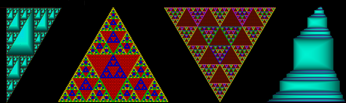
There is a special subset of the
Julia fractals consisting of fractals generated by so-called "Newton's rootfinding method." We call them Newton fractals and discuss them in § 8. Here are sample fractals:


Figure 1.9(A). "Butterflies"


Newton Fractal on a z-Canvas


Figure 1.9(B). "Spiders"


Newton Fractal on a z-Canvas


Figure 1.9(C). "Dragonflies"


Newton Fractal on a z-Canvas


Figure 1.10(A). "Newton Garden"


Newton Fractal on a z-Canvas


Figure 1.10(B). "Firefly Forest"


Newton Fractal on a z-Canvas


Figure 1.10(C). "Crab Shell"


Newton Fractals on a z-Canvas with Different Colorings


Figure 1.10(D). "Barn Owl"


Newton Fractal on a Plane (z-Canvas) and a Sphere


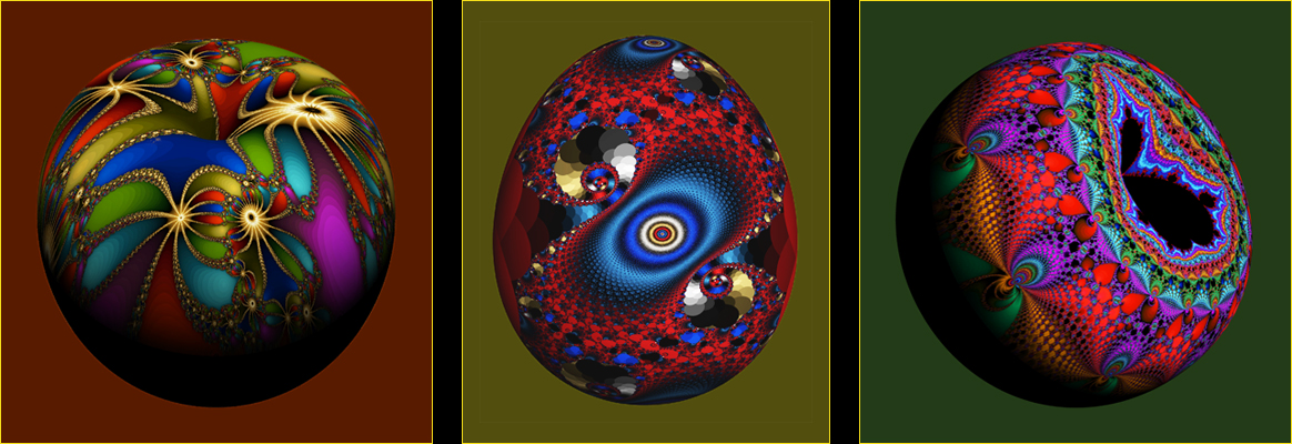
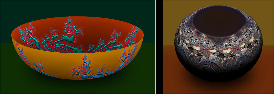
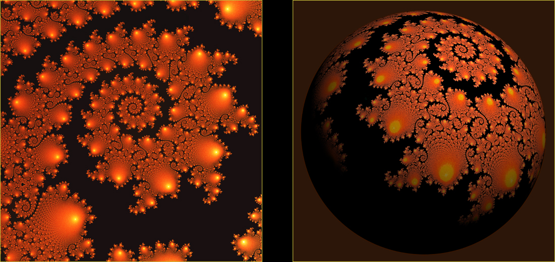
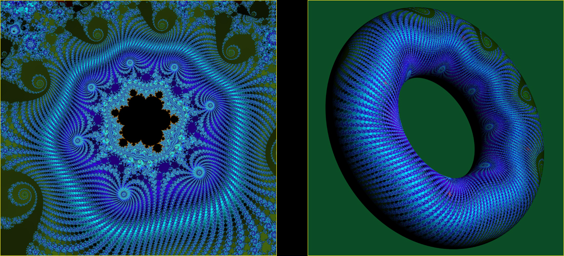
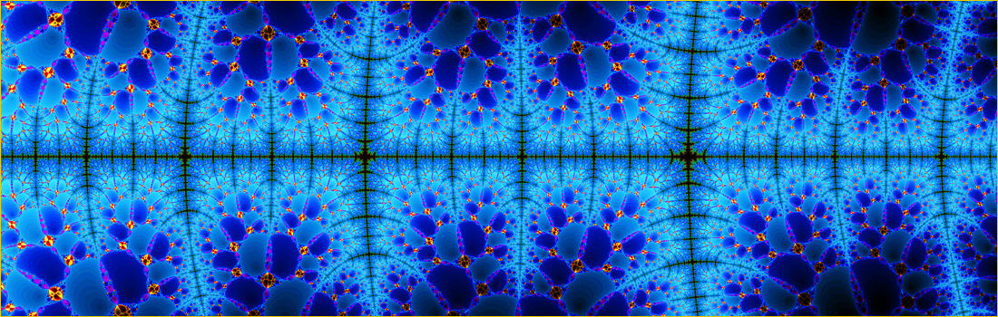
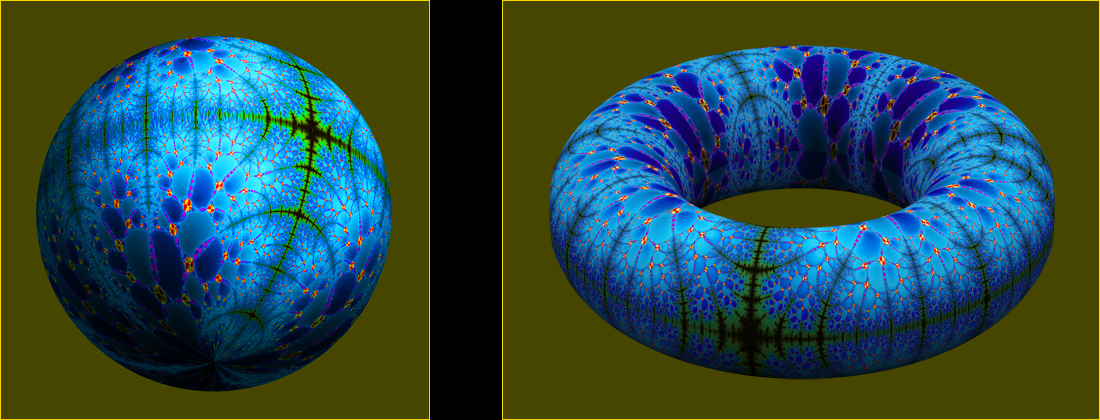
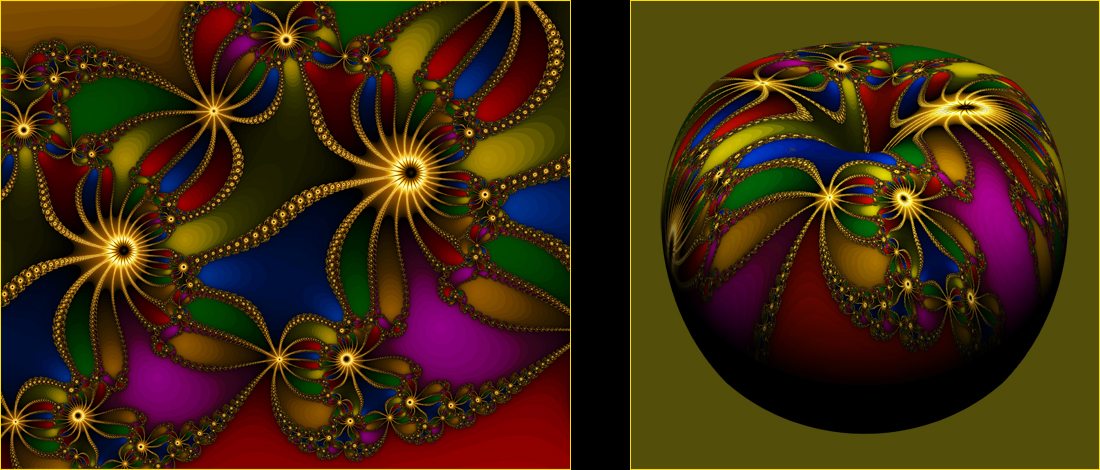
People who are familiar with multivariable calculus can venture into plotting fractals in a 3D space. One of the possibilities is to map a fractal from the plane to various surfaces such as a sphere and a torus. We will throw in 3D examples here and there in the upcoming sections.


Go to   Top of the Page

§ 1. Previews of § 2 - § 8
§ 3. The Mandelbrot Set
§ 6. Generalizations

Fractal Coloring Algorithms
Introduction

§ 2. The Divergence Scheme
§ 4. The Convergence Scheme
§ 7. The Logistic Equation

Gallery 2D
Prep Math


§ 5. Julia Sets
§ 8. Newton Fractals

Gallery 3D


§ 2.  The Divergence Scheme

We say that a sequence zn of complex numbers diverges to ∞ if the real sequence |zn| diverges to ∞, i.e., if zn gets further away from the origin of the complex plane without bound as n gets larger. The object of § 2 is to introduce a fractal plotting technique, called the "Divergence Scheme," associated with the notion of divergence of
orbits of complex parameters p generated by the Mandelbrot equation (1.1).


Figure 2.0. Sample Fractal Generated by the Divergence Scheme


Technical Description: A Local Image of The Mandelbrot Set on a p-Canvas
Centered at p = (0.28212348434375, 0.0110096504375)


We first view the complex plane as the set of all (complex) parameters p, and for each p in the complex plane, define a function fp of a complex variable z by setting fp(z) = z 2 + p. Since p is a constant in each fp, its derivative is fp'(z) = 2 z, hence, its critical point is z = 0. Yes, we can apply the familiar rules of differentiation from elementary calculus on fp. We then write the dynamical system
(1.1) as

(2.1)   zn+1 = fp(zn) = zn2 + p

and set

(2.2)   z0 = 0,

which is the critical point of fp. Thus, for each p, (2.1) together with (2.2) constitutes the
orbit zn of p with the fixed initial value z0 = 0. Because its initial value is the critical point, we call the orbit the critical orbit of p. Throughout § 2 - § 4, we assume, unless otherwise stated, that every orbit zn is a critical orbit of p satisfying (2.1) and (2.2). With that we have the following surprisingly simple definition of probably the best known object in modern mathematics:

The Mandelbrot Set, which we will denote by , means the set of all parameters p in the complex plane whose (critical) orbits do not diverge to ∞.

If a and b are real numbers, let max{a, b} denote the largest of a and b. To develop our fractal plotting method, we need:

Proposition A: Any orbit zn of p (critical or noncritical) diverges to ∞ if and only if |zm| > max{2, |p|} for some m.
Proposition B: If |p| > 2, then the critical orbit zn of p diverges to ∞, i.e., p does not belong to the Mandelbrot set ℳ.


Proof of A: Suppose |zm| > max{2, |p|} for some m. Then by (2.1) and the triangle inequality (see § 1(a)), we have

   |zm+1| = |zm2 + p| ≥ |zm|2 - |p| ≥ |zm|2 - |zm| = |zm|(|zm| - 1) = α|zm|,

where α = |zm| - 1 > 1. Since |zm+1| ≥ α|zm| > |zm| > max{2, |p|}, we may repeat the above argument to get

   |zm+2| ≥ |zm+1|(|zm+1| - 1) ≥ α|zm|(|zm| - 1) ≥ α2|zm|.

By induction, it follows that |zm+k| ≥ αk|zm| for any k ≥ 1. Since α > 1, we conclude that if |zm| > max{2, |p|} for some m then the orbit zn diverges to ∞. The converse of the statement is trivial.

Proof of B: If |p| > 2, (2.1) and (2.2) imply |z1| = |p| > 2; hence, by the triangle inequality (see § 1(a)), we have

    |z2| = |z12 + p| ≥ |z1|2 - |p| = |p|2 - |p| = |p|(|p| - 1) > |p| = max{2, |p|}.

Hence, by Proposition A, the orbit zn diverges to ∞.


Figure 2.1. The Mandelbrot Set


With zm > θ, θ = 2


With zm > θ, θ = 10
Propositions A with |p| ≤ 2 and Proposition B together imply:

The Divergence Criterion:
|zm| > 2 for some m if and only if the (critical) orbit zn of p diverges to ∞.

Here, we note that if |p| > 2 the divergence criterion is trivial because of Proposition B, and if |p| ≤ 2 then max{2, |p|} = 2 in Proposition A. We also note that |p| > 2 means p is outside of the circle with radius 2 and |zm| > 2 for some m means: The orbit zn of p gets out or "escapes" from the circle at some
instant or time n = m.

We now use the divergence criterion and a computer to plot the Mandelbrot set ℳ. Let R be a square canvas comprising 2,000 × 2,000 = 4,000,000 pixels centered at the origin (0, 0) of the complex plane with radius 2, i.e., R is bounded by xmin = -2, xmax = 2, ymin = -2 and ymax = 2. Defining a canvas is always the first step of fractal plotting.

We then regard R as a p-canvas so as to identify each pixel (i, j) in the canvas with a unique parameter p belonging to the pixel.

The Divergence Scheme: Plotting ℳ on the p-canvas is now easy. Paint the entire canvas R, say, white initially, and let M = 1000 and θ = 2. For every pixel (i. j), er, parameter p, in the p-canvas R, iterate (2.1) with (2.2) at most M times and paint the canvas R as follows:

  •   If |z1| > θ then color the pixel p black ,
  • else if |z2| > θ then color the pixel p red ,
  • else if |z3| > θ then color the pixel p black ,
  • · · ·
  • else if |zM| > θ then color the pixel p red .

  • Thus, the above scheme assigns the color, red or black, to each pixel p in the p-canvas R according to how quickly the orbit zn of the parameter p escapes from the circle of radius θ = 2 before taking a long journey toward ∞; see the
    divergence criterion. For example, if p = (2, 0) then |z1| = θ and |z2| > θ, so the "escape time" is m = 2 and the pixel p is colored red.

    We call the plotting process given by the if-statement the divergence scheme, so as to contrast it with the convergence scheme, which we will introduce in § 4.

    Of course, an actual computer program based on the divergence scheme can be streamlined in many ways. Probably the most important is to use |zm|2 > θ2 instead of |zm| > θ to avoid using the hidden square root in |zm| and shorten the computing time as it is used millions, if not billions, of times while running the program.

    Figure 0.1 shown at the outset of this article is the output image of the computer program in which the circle of radius θ = 2 is visible. The portion that retains the white canvas color and resembles a "snowman" figure is precisely an approximation of ℳ plotted on the canvas with finitely many pixels and by replacing ∞ in the definition of ℳ by "up until M = 1000."

    The first of the two images in Figure 2.1 shows a closeup of the approximated Mandelbrot set ℳ.

    Now, simple logic shows that the
    divergence criterion remains true if we replace θ = 2 by any real number θ ≥ 2, and it implies that the divergence scheme is valid for any θ ≥ 2. The second image in Figure 2.1 is given by increasing the "threshold" from θ = 2 to θ = 10. Looking at the red-black stripes of both images, it appears that ℳ is better (albeit marginally) approximated if the threshold θ gets greater.

    In fact, the accuracy of a computer plot by the divergence scheme depends on the size (or image resolution) of the canvas, the maximum number of iterations M and the threshold θ. The computer plot gets more accurate if any of the three gets greater but with "diminished returns" and with the cost of increasing the computing time. We generally keep the threshold low between 2 and 10 and increase M and the canvas size for a better image. The best way of finding good numbers is to engage in frequent trial-and-error computer experiments. It gets easier quickly as it is similar to figuring out the amount of time needed to cook something in a microwave oven. We generally omit mentioning "approximation," understanding that all computer-generated fractal images are approximations of "real" things.

    Figure 2.1(B). The Mandelbrot Set


    Coloring Fractals by 24-Bit Colors:  Modern computers show graphics in the "24-bit colors" comprising 224 ≈ 16 million colors and we can modify the divergence scheme to take advantage of the capacity to plot colorful fractals such as
    Figure 2.0; see Fractal Coloring Algorithms. For example, the image on the left is painted by a basic technique described in the website.

    Figures 2.1 and 2.1(B) show that the divergence scheme paints the
    complement of ℳ while leaving ℳ in a single canvas color like white and black.

    Basic
    Topological Properties of the Mandelbrot Set ℳ:Proposition B implies that ℳ is enclosed in the circle of radius 2 so it is bounded. It can be also shown that ℳ is closed, i.e., it contains its boundary as its subset. Therefore, ℳ is compact. Note that the boundary of ℳ is the boundary of the complement of ℳ as well.

    Zooming In On Local Images: Even though the images in
    Figure 2.1 are painted in a primitive way that uses only three colors, it gives us valuable information about ℳ. For example, the red-black stripes in the images get more and more complex when they get nearer the boundary of ℳ. What kind of world do we have in the area that is extremely close to the boundary of ℳ ?

    The question leads to our common practice of zooming in on a small rectangular neighborhood of a point extremely near or on the boundary of ℳ. Here, the sides of the small rectangle are parallel to the coordinate axes of the complex plane so we can use the rectangle as a canvas with a large number of pixels to magnify the "local" image by the divergence scheme.

    Example 1:  The image shown below on the left is a local image of ℳ given by zooming in on the microscopic square neighborhood of the complex parameter p = (-0.688497, 0.279885) with radius 0.000073. p is very near or on the
    boundary of ℳ but not in the interior of ℳ. It is generated by the divergence scheme with the coloring technique similar to the one used to paint the "global" Mandelbrot set shown in Figure 2.1(B). The global image hides infinitely many intricate local images and we try to get them like treasure hunters.


       Figure 2.2. A Local Image of ℳ Generated by the Divergence Scheme


    People familiar with multivariable calculus can find a fun project of painting the fractal on a nonplanar surface like a sphere.

    Example 2:  Figure 2.3 is a cropped and resized image from a computer plot on the large square p-canvas with 6,400 × 6,400 pixels centered at the complex number (0.28206125, 0.011014375) with radius 0.0000011. M = 100,000 is used as the maximum number of iterations for the divergence scheme. The image contains several (deformed) replicas of the "snowman" painted black, which we call mini-Mandelbrot sets. They look like small isolated islands but as we'll find out in the next section, they are actually connected to ℳ by razor-thin "filaments" belonging to the
    boundary of ℳ.


    Figure 2.3.  Another Local Image of the Mandelbrot Set


    The zooming process can be repeated on the local image to capture additional local images. It is time consuming to compute a fractal on such a large canvas, but it gives us an option of finding additional local images as well as an option of making a high resolution printout of the image. For example,
    Figure 0.5(C) is given by zooming in on microscopic rectangles in Figure 2.3 and applying the divergence scheme.

    This and That:  (1) Here, we show that the zooming process is fairly easy. Use graphic software such as Photoshop and place the mouse cursor on the point on the image like Figure 2.3 we want to zoom in on and get its pixel coordinates (i, j). Then use the
    conversion formulas (1.2) and (1.3) to convert the pixel coordinates (i, j) to the Cartesian coordinates (x, y) like (0.28122928, 0.01134422). This can be done by a simple computer program.

    (2) It is not too hard to generalize the divergence criterion and find a threshold like θ = 2 for a general polynomial dynamical system. We have also seen that any number θ ≥ 2 can be used as a threshold for the divergence scheme with possibly an improved output image. This provides us with a nice tool for computer experiments, when we use a polynomial dynamical system other than the Mandelbrot equation and want to avoid calculating a threshold. But be careful: Blindly increasing the threshold also increases the computing time without notably improving the output image. There is a good reason why Mandelbrot used the smallest threshold θ = 2 in plotting the Mandelbrot set when the computers were much slower.

    Multibrot Set:  A Multibrot set is a straightforward extension of the Mandelbrot set given by the Mandelbrot equation (2.1) with 2 replaced by an integer k ≥ 2. For example, shown below is a local image of the Multibrot set with k = 7 given by the seventh degree Mandelbrot equation

    (2.3)   zn+1 = fp(zn) = zn7 + p

    with z0 = 0 painted on a plane and a torus.


    Figure 2.4.  Seventh Degree mini-Mandelbrot Set


    Go to   Top of the Page

    § 1. Previews of § 2 - § 8
    § 3. The Mandelbrot Set
    § 6. Generalizations

    Fractal Coloring Algorithms
    Introduction

    § 2. The Divergence Scheme
    § 4. The Convergence Scheme
    § 7. The Logistic Equation

    Gallery 2D
    Prep Math


    § 5. Julia Sets
    § 8. Newton Fractals

    Gallery 3D

    .

    § 3.  The Mandelbrot Set

    Recall that the Mandelbrot set is denoted by ℳ and is
    closed so it contains its boundary as its subset. It is also known that the topological dimension of the boundary is 1 like the boundary of a circular disk, so we intuitively picture it as an object made of "razor-thin filaments" without thickness. Does it mean that the area of the boundary is zero? Nobody can find the answer, and we suddenly realize that it is considerably more complex than it appears in a global image like Figure 2.1.

    Although it may not sound obvious unless we know something about
    fractal dimensions, the following celebrated theorem implies that no figures on the plane are more complex than the boundary of the Mandelbrot set, boosting the Mandelbrot set to be one of the most complex objects ever plotted on a plane.

    Shishikura's Theorem (1998): The fractal dimension of the boundary of the Mandelbrot set is 2 (which is the topological dimension of the plane).


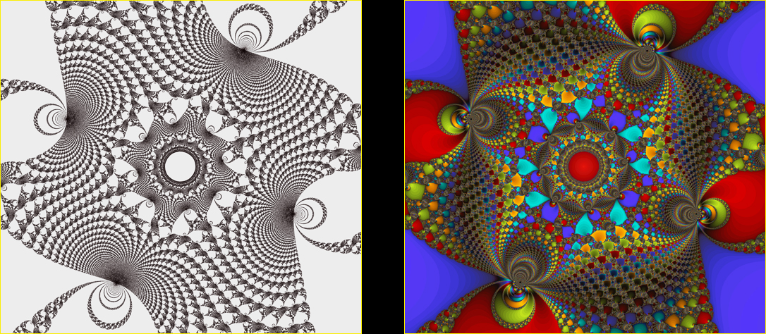
    Let's pause for a moment and look at its local image in, say, Figure 2.3, in which a part of ℳ is visible. The intricate image surely looks impressive, but exactly where is the boundary of ℳ and what does it have to do with the colorful patterns? It turned out that the boundary of ℳ is all over the image as we can see in Figure 3.1 given by darkening the entire Figure 2.3 and lighting up its razor-thin filaments:


    Figure 3.1.  The Boundary of the Mandelbrot Set in Figure 2.3


    The image shows that the boundary of ℳ in the rectangular area is vividly self-similar, making it a fractal as per our informal definition. Shishikura's theorem also makes it a fractal according to Mandelbrot's definition: A fractal means a set for which the Hausdorff-Besicovitch dimension (aka the fractal dimension) strictly exceeds the topological dimension. Through the self-similarity of indefinitely repetitive patterns, we observe that the luminous filaments of the boundary of ℳ get so dense they work like space-filling curves in infinitely many areas of the plane. It provides us with an intuitive idea as to why the "fractal dimension" of the boundary of ℳ is the same as the topological dimension of the plane.

    Fractal dimensions in fact measure complexities and space-filling capacities of any curves (i.e., objecs of topological dimension 1) by fractional scales between 1 and 2, and the boundary of ℳ attains the maximum value of 2 per Shishikura's theorem. By comparison, the fractal dimension of the boundary of the "Koch Snowflake" shown in Figure 0.4 is 1.2619. It should be noted in the aforementioned Mandelbrot's definition of fractal that the fractal dimension of the boundary of ℳ also exceeds its topological dimension by the largest possible value.

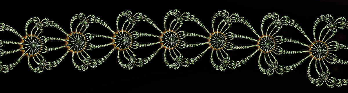
    The boundary image of
    Figure 3.1 also shows that it works like the basic monochromatic line art of the multicolored ukiyo-e woodblock prints, which are completed by the additional steps of coloring between the lines. The finer the line art, the more elaborate the final ukiyo-e print; see Figure 0.6(A).


    Another Local Image of ℳ and its Boundary (Right)


    This is another local image of Figure 2.3.


    One of the most important
    topological properties in fractal geometry is "connectedness" of a set and Figure 3.1 appears to show that the Mandelbrot set ℳ with its complex boundary is "connected" as "one piece." To give precision to the intuitive concept involving "one piece," R. C. Buck adopts the following formal definition in his classical textbook for Advanced Calculus: Suppose S is a nonempty set of points in the xy-plane. S is said to be connected if it is impossible to split S into two disjoint sets, neither one empty, without having one of the sets contain a boundary point of the other.

    For example, it is known that the "neck" of the "snowman" in Figure 2.1 is the point (-3/4, 0), and if we cut the head off the body of the snowman with the vertical line x = -3/4, then either the head or the body contains the boundary point of the other, namely (-3/4, 0). Thus, the particular attempt fails to show that ℳ is disconnected. Because of the complexity of its boundary, proving whether or not ℳ is connected is by no means a simple task, as evidenced by the fact that Mandelbrot initially conjectured ℳ to be disconnected and reversed it later without substantiation―before Adrien Douady and John H. Hubbard settled it:

    The Douady-Hubbard Theorem (1982): The Mandelbrot set is connected.

    They also proved that ℳ is "simply connected," which means ℳ has no holes. Topologically speaking therefore, ℳ is well-behaving as a
    compact set in one piece without a hole. As described by Wikipedia, Douady and Hubbard established many of the fundamental properties of ℳ at an early stage and created the name "Mandelbrot set" in honor of Mandelbrot. They were the pioneers of the mathematical study of ℳ.

    "Who Discovered the Mandelbrot Set?" is the title of an interesting read that appeared in Scientific American in 2009. It writes: Douady now says, however, that he and other mathematicians began to think that Mandelbrot took too much credit for work done by others on the set and in related areas of chaos. "He loves to quote himself," Douady says, "and he is very reluctant to quote others who aren't dead."


    Figure 3.2.  "Daytime" and "Nighttime Views" of a Fractal


    Local Images of ℳ in a Neighborhood of p = (0.28212348434375, 0.0110096504375)


    "Daytime" and "Nighttime Views" of a Fractal:  Shown above on the left is another fractal generated by the Mandelbrot equation (2.1) and the divergence scheme, where the razor-thin filaments of the boundary of the Mandelbrot set ℳ are invisible. When its colors are darkened and the thin filaments are lit up, we get the "nighttime view" of the fractal on the right, vividly showing the presence of the complex boundary of ℳ hidden in the "daytime view" on the left.

    Note that the two views may appear totally different, mainly because the daytime view shows the
    complement of ℳ. Figure 2.3 we have seen is a daytime view while Figure 3.1 is a nighttime view. The nighttime views are not as colorful but they make it easier for us to visualize the important theorems established by Shishikura, Douady and Hubbard.

    Plotting the complex boundary of ℳ with reasonable accuracy may demand weeks of computing time even with a fast modern computer. Figure 3.3 shown below is a resized and cropped image from a fractal on the p-canvas with 4,000 × 4,000 pixels centered at the point

    p = (0.25000316374967, -0.00000000895972)

    with a microscopically small radius ≈ 0.0000000000003 = 3 × 10-13.  We note that p is very near the cusp (0.25, 0) of the cardioid in
    Figure 2.1.


    Figure 3.3.  A mini-Mandelbrot Set under the Microscope


    M = 1,500,000 M = 500,000


    For the above image on the left, we used whopping 1,500,000 iterations of the Mandelbrot equation for each black pixel. If we use M = 500,000 (still a large number) instead, the outline of the mini-Mandelbrot set becomes blurry as shown in the above picture on the right. Fortunately, computers (especially used ones) are inexpensive nowadays and we can easily afford a second or third computer to do tedious jobs. Programming carefully so as to minimize computing time is not as important as it used to be. Shown below is a nighttime view of the fractal on the left that reveals the boundary of the mini-Mandelbrot set.


    Figure 3.4.  The Boundary of the mini-Mandelbrot Set


    Topological Properties
    (continued): We stated earlier the precise definition of a set being "connected" as "one piece" and now wish to dig into the notion of "pieces" as a preparation for the upcoming sections. We showed, while discussing the definition by Buck, that the "snowman" of Figure 2.1 cannot be split into "two pieces," the head and body, without having either one of them contain a boundary point of the other.

    If we restrict our attention to the interior of ℳ which does not contain any of the boundary points, the situation changes completely. Not only can we split the head from the body without worrying about the boundary points, we can actually decompose the snowman into numerous disjoint connected body parts including all those (circular) disks attached to the cardioid body. Note that each of the disks is an open set without a boundary point and it is maximal in the sense that it is not a proper subset of a larger connected subset of the interior of ℳ.

    In general, if S is any nonempty set of points in the complex plane, a nonempty maximal connected subset of S is called a connected component of S. It is easy for people familiar with elementary set theory to use the idea of an "equivalence relation" and prove that S can be partitioned into the disjoint union of its connected components. Thus, S is connected if and only if it consists of exactly one connected component (or "piece"). By virtue of the Douady-Hubbard theorem, ℳ has exactly one connected component, but its interior is disconnected and has infinitely many connected components including the aforementioned open disks.

    The set S is said to be totally disconnected if it is disconnected and every connected component of S comprises just one point. As we'll see, many fractals are totally disconnected, but the interior of ℳ is not one of them.

    Compactness, connectedness, the number of connected components, being simply connected without a hole and being totally disconnected are all topological properties. Topologists generally identify homeomorphic objects and use topological properties to distinguish objects. In the 3D space, for example, a donut and a coffee cup with a handle are the same to topologists but the "broken taiko drum" shown below and a ping pong ball are different.


    "Broken Taiko Drum"

    Here, we have the mini-Mandelbrot set of Figure 3.3 flipped vertically and painted in different colors and its application in multivariable calculus.


    Go to   Top of the Page

    § 1. Previews of § 2 - § 8
    § 3. The Mandelbrot Set
    § 6. Generalizations

    Fractal Coloring Algorithms
    Introduction

    § 2. The Divergence Scheme
    § 4. The Convergence Scheme
    § 7. The Logistic Equation

    Gallery 2D
    Prep Math


    § 5. Julia Sets
    § 8. Newton Fractals

    Gallery 3D


    § 4.  The Convergence Scheme

    We are not done yet with the complex nature of the Mandelbrot set ℳ and still stay with it. In § 2 and § 3, we discussed the
    complement and the boundary of ℳ; see "Daytime and Nighttime Views" of a Fractal. We now turn our attention to its interior, namely, ℳ minus its boundary.

    The Mandelbrot set has become so illustrious, everybody interested in fractals knows its "snowman" shape by heart. To its main body, which is a heart-shaped "cardioid," a bunch of (circular) disks are tangentially attached, and to each of these disks another bunch of disks are tangentially attached; see "Mandelbrot Set" by Wikipedia for detail. The fractal pattern repeats as if the cardioid has children, grandchildren, great grandchildren and so on and so forth. Here, a "cardioid" means, instead of the familiar curve, the curve together with all the points inside the curve.

    As
    Figure 3.1 shows, ℳ also contains infinitely many mini-Mandelbrot sets, each of which is a smaller copy of ℳ, again comprising a cardioid (which may be distorted) with infinite generations of disks (which may be distorted) and even smaller mini-Mandelbrot sets. If we remove the boundary of ℳ from ℳ, we are left with the interior of ℳ comprising the interiors of these disks and cardioids, etc., which are, as we have discussed, the connected components of the interior of ℳ.

    Atoms and Molecules: Let's use Mandelbrot's idea shown in his article as a cue and call each connected component of the interior of ℳ an atom of ℳ and a (disjoint) union of one or more atoms a molecule. Thus, atoms include the interiors of all those disks and cardioids with various degrees of distortion and possibly other shapes we have not recognized. An atom and the interior of a mini-Mandelbrot set are examples of molecules.

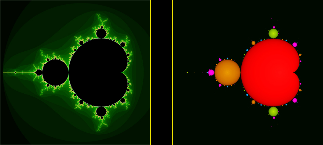
    As we saw in § 2, the divergence scheme cannot distinguish these atoms and paints them in a single color like black or white. Our current goal is to develop another simple algorithm called the convergence scheme which will be used to color ℳ like in Figure 4.1 and many other fractals in upcoming sections. Along the way, we will see that the atoms are associated with "periods" like in chemistry (but in a totally different way).


    Figure 4.1.  The Mandelbrot Set with Colorful Atoms


    Cycles and Periods: A sequence cn of complex numbers is called a cycle if there is a positive integer k satisfying cn = cn+k for any index n. The smallest such integer k is called the period of the cycle, and a cycle with period k is called a k-cycle for short. For example, the sequence

        1, 2, 3, 1, 2, 3, 1, 2, 3, 1, 2, 3, 1, 2, 3, 1, 2, 3, · · ·

    is a 3-cycle but not a 6-cycle or a 9-cycle. The sequence  0, 0, 0, 0, · · ·  is a 1-cycle, which we identify with the constant 0.

    A sequence zn is said to converge to a k-cycle cn provided that zn gets arbitrarily close to cn as n gets bigger, or more precisely, for any real number ε > 0, there is an integer N > 0 such that n ≥ N implies |zn - cn| < ε.  For example, the sequences  1/2, 1/3, 1/4, 1/5, 1/6, · · ·  and  1/2, 2/3, 3/4, 4/5, 5/6, · · ·  converge to the constants 0 and 1, or equivalently, to the 1-cycles 0, 0, 0, 0, · · ·  and  1, 1, 1, 1, · · ·,  respectively. Therefore, the sequence

        1/2, 1/2, 1/3, 2/3, 1/4, 3/4, 1/5, 4/5, 1/6, 5/6, · · ·, 1/1000, 999/1000, 1/1001, 1000/1001, · · ·

    converges to the 2-cycle 0, 1, 0, 1, 0, 1, 0, 1, 0, 1, · · ·, 0, 1, 0, 1, · · ·.

    Figure 4.2. The Convergence Scheme


    With k = 1


    With k = 1, 2, 3, 4


    With k = 1, 2, 3, ..., 90

    Again, suppose ε is a (small) positive real number. Using the aforementioned definition of a k-cycle and the
    triangle inequality, it is easy to prove the following.

    Proposition:  If a sequence zn converges to a k-cycle then there is a positive integer N such that for all n ≥ N, |zn+k - zn| < ε.

    The Convergence Scheme: Our new algorithm called the convergence scheme with period index k is based on this proposition and given by replacing the inequality |zm| > θ  of the
    red-black divergence scheme of § 2 by the inequality |zm+k - zm| < ε. Thus, for each pixel (i, j), er parameter p, on the p-canvas R and its (critical) orbit zn, it is given by the if-statement:

  •   If |z1+k - z1| < ε then color the pixel p col1,
  • else if |z2+k - z2| < ε then color the pixel p col2,
  • else if |z3+k - z3| < ε then color the pixel p col3,
  • · · ·
  • else if |zM+k - zM| < ε then color the pixel p colM.

  • Here, col1, col2, ... , colM are prescribed colors and ε a small positive real number like 10-6, Δx or Δy; see
    (1.2). ε works like the threshold θ of the divergence scheme, except that the output image is more accurate when ε is smaller.

    For simplicity, let's call a parameter whose critical orbit converges to a k-cycle a parameter of period k and call an
    atom an atom of period k if it comprises parameters of period k. With that we have:

    Example 1 (The Mandelbrot Set): Start with the p-canvas R, which is the rectangle in the complex plane with center (-0.52, 0) and horizontal radius 1.65 and comprises 3,000 × 2,500 pixels.

    We first apply the divergence scheme with M = 20000 and θ = 2 on R and extract the Mandelbrot set ℳ comprising the pixels p whose orbits do not diverge to ∞. Then apply various convergence schemes with ε = 10-8 on ℳ. Figure 4.2 shows the (resized) output images of three molecules.

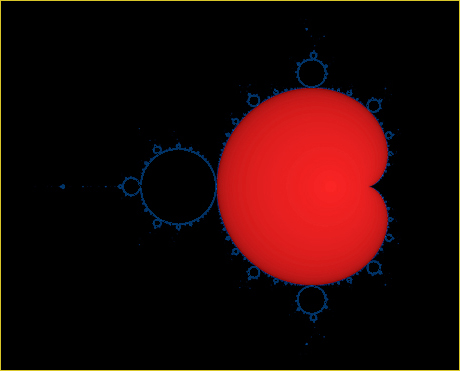
    The first image is generated by the convergence scheme with period index k = 1 and shows that the interior of the cardioid is an atom of period 1. Painting in subtle shades of red is done by a basic technique included in the Fractal Coloring site.

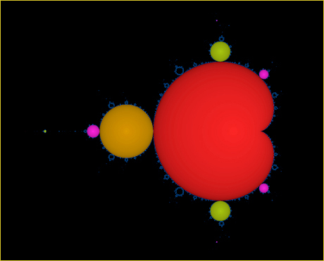
    The second image is given by the convergence scheme with period indices k = 1, 2, 3, 4, which is basically defined as the natural sequence of the four convergence schemes, the one with period index k = 1 followed by the one with period index k = 2, etc. It shows that the interior of the largest disk is an atom of period 2 and painted in subtle shades of orange. Similarly, the green and purple atoms are of periods 3 and 4, respectively.

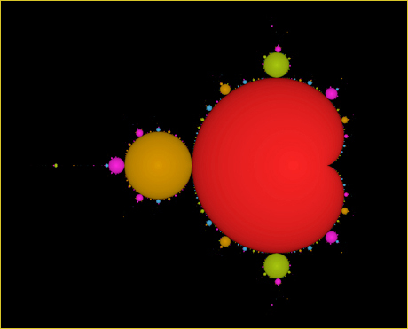
    The third image is given by a straightforward extension of the scheme described in the preceding paragraph. Because there aren't enough colors that are easily distinguishable, the correspondence between the periods and colors of the atoms is not one-to-one. For example, the atoms of periods 2 and 5 are painted orange in the third image.

    Example 1 shows that the convergence scheme may mean the one with a single period index or multiple period indices. Note that the convergence scheme with, say, period index 6 cannot distinguish parameters of periods 1, 2, 3 and 6 that are divisors of 6. Therefore, we need to be a little careful when we program a computer to carry out the convergence scheme, especially the one with multiple period indices.

    Mini-Mandelbrot Sets: Recall that the last image of Figure 4.2 is painted on a large canvas, and it includes the parts given below in Figure 4.3. The closeup images show not only meticulously aligned circular atoms but also several molecules that look like little flying insects. Looking at his computer printout of ℳ created by a dot matrix printer of the 1970s, Mandelbrot initially thought they were "dirt."

    The dirt turned out to be well structured molecules that look like smaller copies of ℳ. Because such copies play
    important roles in fractal art, we define a mini-Mandelbrot set to be a molecule ℳ ' satisfying the following two conditions: (a) there is a one-to-one correspondence between the atoms of ℳ and the atoms of ℳ ', and (b) there is an integer λ ≥ 2 such that for every atom of ℳ ', its period is given by

    (4.1)  λ k ,

    where k is the period of the corresponding atom of ℳ. We call λ the period of ℳ '.

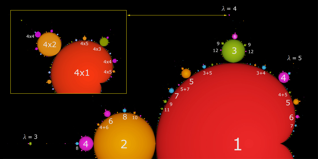
    For example, the most visible mini-Mandelbrot set of Figure 4.3 happens to have period λ = 4 and is shown in Figure 4.4 and the inset of the periodicity diagram. There, it is painted by the convergence scheme with period indices λ k = 4, 8, 12, ..., 100 and with the colors of the Mandelbrot set of Figure 4.2 so as to emphasize the one-to-one correspondence between the atoms of ℳ and the atoms of the mini-Mandelbrot set.


    Figure 4.3.  Closeups of the Interior of the Mandelbrot Set


    Figure 4.4 shows that the boundary of the mini-Mandelbrot set of period λ = 4 is more intricate than the boundary of the Mandelbrot set seen in
    Figure 4.1. In fact, computer experiments seem to indicate that every copy of ℳ we encounter is a mini-Mandelbrot set, which is associated with a period λ in such a way that the greater the period, the more intricate the surrounding pattern of the mini-Mandelbrot set. Gallery 2D shows an application of certain types of mini-Mandelbrot sets in fractal art.

    Here's an additional technical detail: For the convergence scheme with period indices λ k = 4, 8, 12, ..., 100, we used the variable maximum number of iterations

    (4.2)  M = 20000 - 150k,

    rather than a constant like M = 20000 to speed up the computation without notably sacrificing the appearance of the output image.


    Figure 4.4.  The the mini-Mandelbrot Set of Period λ = 4 and Its Boundary


    Weakness of the Convergence Scheme: The convergence scheme with period index k is slow especially when k is large. That's mainly because it uses |zn+k - zn| < ε to test if zn reached the
    threshold (instead of |zn| > θ in the divergence scheme), which requires up to k × M extra iterations of (2.1) for each pixel on the canvas belonging to ℳ.

    Aside from its aforementioned slowness, the convergence scheme may have a potential issue as it relies on the proposition whose converse is false (unlike the divergence criterion on which the divergence scheme is based). For the convergence scheme to be fully applicable on the interior of ℳ, the critical orbit of every parameter in the interior of ℳ has to be convergent to some cycle, thereby satisfying the hypothesis of the proposition. The next two paragraphs address this issue.

    Ghost Atoms: Recall that an
    atom of the Mandelbrot set ℳ is by definition a connected component of the interior of ℳ and that every atom we have dealt with seems to have a period k, i.e., it comprises parameters whose critical orbits converge to a k-cycle for some k; see the periodicity diagam. Any other type of atom is called a ghost atom (or "ghost component" per Wikipedia) as its existence or nonexistence has not been proven.

    Famous Conjecture and the Validity of the Convergence Scheme: It has been conjectured that ghost atoms do not exist; see
    density of hyperbolicity. It implies that every parameter in the interior of ℳ has the critical orbit that converges to a cycle, satisfying the hypothesis of the proposition.

    Chaos in the Mandelbrot Set: In general, a critical orbit either diverges to ∞ or converges to a cycle, or else it is called a chaotic orbit. Because of the conjecture and the fact that the complement of ℳ comprises the parameters whose orbits diverge to ∞, the parameters with chaotic orbits fall into the boundary of ℳ. It is also
    known that the orbit of each parameter p in the boundary of ℳ reacts sensitively to a minuscule change of the value of p and totally alters its behavior. In other words, the boundary is where chaos occurs in the Mandelbrot set.

    We now know that the convergence scheme is valid for painting the interior of ℳ. What happens if we apply the convergence scheme on the complement of ℳ ?


    Figure 4.5.  The Eyeball Effect (Right) Given by the Convergence Scheme


    The "Eyeball Effect": The following is a testament that even a programming bug can create a beautiful output image sometimes and help us discover interesting ideas. The picture shown above on the left is essentially the same as
    Figure 3.3 (but in different colors) and is given by the divergence scheme alone, while the one on the right is painted by the divergence scheme followed by the convergence scheme with period index k = 1 (using different colors) on the complement of ℳ. The "eyeballs" painted by the convergence scheme are caused by its "mistake" of confusing some of the slowly divergent orbits as convergent. The images show which parameters are affected. Figure 1.8(D) and Figure 5.8 illustrate the "eyeballs" more vividly.

    Artist's Rendering: We have seen a plain approximation of the Mandelbrot set ℳ in an image like
    Figure 2.1 and a more colorful version in Figure 4.1. The latter should probably be called an artist's rendering of ℳ rather than an approximation, as the convergence scheme allows us to illustrate ℳ in many varieties of ways. Here are additional artist's renderings of ℳ.


    Figure 4.6.  "Mandelbrot Platters"


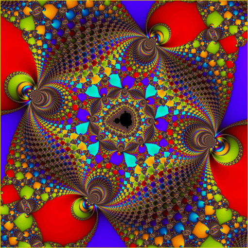
    Periodicity Diagram: If we label the atoms of the Mandelbrot set in
    Figures 4.2 and 4.4 by their periods instead of colors, we get the following periodicity diagram. The periods in the diagram show meticulously aligned numerical patterns that are easy to recognize and will play an important role in plotting many of the "Julia sets" in the next section. The numerical patterns are yet another amazing property of the Mandelbrot set ℳ.


    Figure 4.7.  Periodicity Diagram of ℳ


    Note: λ is the period of a mini-Mandelbrot set


    Go to   Top of the Page

    § 1. Previews of § 2 - § 8
    § 3. The Mandelbrot Set
    § 6. Generalizations

    Fractal Coloring Algorithms
    Introduction

    § 2. The Divergence Scheme
    § 4. The Convergence Scheme
    § 7. The Logistic Equation

    Gallery 2D
    Prep Math


    § 5. Julia Sets
    § 8. Newton Fractals

    Gallery 3D


    § 5.  Julia Sets

    We have so far viewed the complex plane as the set of parameters p and the Mandelbrot equation
    (2.1) as the collection of all orbits of p varying through the complex plane while the initial value z0 is fixed at the critical point z0 = 0 of the function fp. As shown in § 2, we use these critical orbits to define the Mandelbrot set , which possesses the dazzling features we have witnessed so far.

    In this section, we will show, as yet another fascinating attribute of the Mandelbrot set , that almost every parameter p on or near gives rise to an intricate fractal called the "Julia set" of p. Doing so also reveals, as we'll see, the root of the famed Mandelbrot set and explains why the critical orbits are used in its computation.

    We now view the complex plane as the set of all possible initial values z0 for the Mandelbrot equation

    (5.1)  zn+1 = fp(zn) = zn2 + p,

    while keeping the value of p fixed at a constant.
    Recall that the orbit of p with an initial value z0 is also called the orbit of z0 with the parameter value p. Define the filled-in Julia set of p to be the set of all initial values z0 in the complex plane whose orbits (with the fixed value of p) do not diverge to ∞. Because the definition of the filled-in Julia set is almost identical to the definition of ℳ, we expect that the divergence and convergence schemes are again effective in plotting the filled-in Julia sets, this time on a z-canvas instead of a p-canvas. The use of these plotting schemes is explained in detail in Fractal Coloring Algorithms.

    If p is a parameter in the interior of then p belongs to a unique atom of as shown in the preceding section, so it makes sense to say that the filled-in Julia set of p is "born" from such an atom of ℳ.


    Figure 5.1(A).  "Hydra of Lerna with 11 Heads" Born from an Atom of Period 11


    "Hydra" is an artist's rendering of the filled-in Julia Set.


    Example 1: The "hydra" of Figure 5.1(A) shown above is the filled-in Julia set of the parameter p = (-0.692712, 0.273012) chosen from a circular
    atom of period 11. The atom belongs to the first image of Figure 4.3 and is attached to the red cardioid of the Mandelbrot set. The "hydra" is painted on a z-canvas centered at the critical point z0 = 0 of the function fp by the convergence scheme with period index k = 11 and the background by the divergence scheme with the threshold

          θ = max{2, |p|} = 2;  cf. proposition A.

    It is another fascinating fact about the Mandelbrot set that the period of the parameter p is always reflected in the shape of the filled-in Julia set of p, as in the number of "Hydra's heads," although why it is so is not completely understood.

    Remark on Plotting the Filled-in Julia Set: Recall that the center of the z-canvas used in the example is the critical point z0 = 0 of the function fp, whose orbit coincides with the critical orbit of p. Because the period of p is 11, the critical orbit converges to a cycle of period 11 at the center of the canvas. Therefore, the convergence scheme with period index k = 11 is a natural choice in decorating the filled-in Julia set of Example 1. The shape of the filled-in Julia set reveals interesting dynamics of the orbits affected by the behavior of the critical orbit. Here are additional examples:


    Figure 5.1(B) "Medusa Lion"
    Born from an Atom of Period 10
    Figure 5.1(C) "Medusa Lion"
    Born from an Atom of Period 21


    "Medusa lions" are (artist's renderings of) the filled-in Julia Sets;
    The atoms of Periods 10 and 21 are attached to the red cardioid near its cusp.


    By a Cantor set or Cantor dust we mean a
    totally disconnected set with infinitely many components and a fractal structure. It was named after Georg Cantor, the pioneer of set theory, who discovered the early form of the fractal in 1883.

    Example 2:  The filled-in Julia set of p = (-0.6891, 0.27896) called "Hydra's Ash" in Figure 1.6(C) is a Cantor set. The parameter p happens to be near the aforementioned atom of period 11 but lies outside of the Mandelbrot set. We'll see the reason why it caused the set to be totally disconnected.

    By the Julia set of p, we mean the boundary of the filled-in Julia set. The filled-in Julia set is known to be compact, hence, it contains the Julia set as its subset. Like the boundary of the Mandelbrot set, the Julia set dictates the shape and complexity of the filled-in Julia set and has a strong association with chaos. It is named after Gaston Julia, who was one of the pioneers of fractals generated by dynamical systems along with Pierre Fatou.

    In fractal art, we call a fractal painted on a z-canvas a Julia fractal and it is usually given by a monochromatic Julia set and additional coloring that fills the space defined by the Julia set; see Figure 0.6. For example, the "hydra" of Figure 5.1(A) is a Julia fractal comprising the Julia set that dictates the shape of the "hydra," the background painted by the divergence scheme and the interior of the "hydra" painted by the convergence scheme.
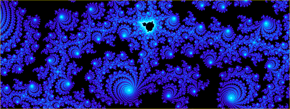

    Figure 5.1(D). The Julia Set of p = (0.25000316374967, -0.00000000895972)


    Example 3:Figure 5.1(D) shows a highly chaotic Julia set of p belonging to the interior of the mini-Mandelbrot set of
    Figure 3.3. Because the period of p is large and unknown, Figure 5.1(E) is painted by the divergence scheme alone on a z-canvas centered at the critical point z0 = 0 and shows the complement of the filled-in Julia set; see the daytime view of the fractal. To our eyes, therefore, the filled-in Julia set is identical to the Julia set of Figure 5.1(D) as its interior is invisible in either figure. If we zoom in on a microscopic neighborhood of the center of Figure 5.1(E), we see a part of the interior of the filled-in Julia set; see the "black hole" of Figure Figure 5.9.


    Figure 5.1(E). "Cuttlefish Lion"

    "Cuttlefish Lion" is not a filled-in Julia set.


    Brief History of the Mandelbrot Set: Fatou and Julia independently established the
    Fatou-Julia theorem in 1919 and amazingly created fractals generated by various dynamical systems using their imaginations instead of computers. The Julia sets representing their fractals, therefore, precede the Mandelbrot set by sixty years. History tells us that the most consequential theorem regarding the Julia sets generated by the dynamical system (5.1) is an immediate corollary to the Fatou-Julia theorem called

    The Fundamental Dichotomy: For any parameter p in the complex plane, the Julia set of p is either connected or a totally disconnected Cantor set.

    For example, the Julia set of Figure 1.1(A) is neither connected nor totally disconnected and the dichotomy assures us that a Julia set like this never arises from (5.1). Mandelbrot, who once studied under Gaston Julia and later became an "IBM fellow," wanted to use a computer and visualize the dichotomy dividing up the complex plane into two parts. So, he initially defined:

    The set ℳ (later named the "Mandelbrot set" by Douady and Hubbard) means the set of all parameters in the complex plane whose Julia sets are connected.

    He knew how to compute ℳ as he was familiar with the Fatou-Julia theorem that clearly implies the Julia set of p generated by (5.1) is connected if and only if the critical orbit of p does not diverge to ∞; see the computer-friendly
    definition of § 2. Thus, the famed Mandelbrot set ℳ was born from the dichotomy of the Julia sets and the rest is history. As we know, the dazzling features and complexities of ℳ extend way beyond whether the Julia sets are connected or totally disconnected.

    Remarks: We call the aforementioned Mandelbrot's definition the alternative definition of the Mandelbrot set. The fact that it is equivalent to our earlier definition explains why the critical point of (5.1) is indispensable in computing ℳ. The Julia sets (and filled-in Julia sets) of Figures 5.1(A)(B)(C)(D) are connected as their generating parameters belong to ℳ while the Julia set (and the filled-in Julia set) of Figure 1.6(C) is a Cantor set.


    Figure 5.2.  "Cloisonné Lion"


    Example 4:  The Julia fractal shown above is a fractal art based on the Julia set of p = (0.2514122, 0.000094) chosen from outside of ℳ near its cusp p = (0.25, 0). Hence, the Julia set is a Cantor set according to the
    alternative definition of ℳ.

    Example 5:  The filled-in Julia sets called "Twin Lions" and shown below are given by parameters belonging to an atom of period 85 = 17 × 5. The atom is attached to an atom of period 17 which is attached to the main cardioid of the Mandelbrot set near its cusp (0.25, 0); see the
    periodicity diagram. Note that both factors 17 and 5 are clearly visible in the "Twin Lions."

    The two "lions" are painted by the convergence scheme with period index 85 and the background by the divergence scheme with the threshold θ = 2. The curling directions of the mane of the "Twin Lions" are opposite to each other and depend on the locations of the parameters in the atom.


    Figures 5.3 & 5.4.  "Twin Lions" born from the same atom of period 17 × 5


    Example 5 (Continued): "
    Esmeralda Lion" with a technical description in Gallery 2D is an enlarged version of the filled-in Julia set shown above on the left. "Ruby Lion" shown below is an enlarged version of the filled-in Julia set shown above on the right.


    Figure 5.5.  "Ruby Lion"


    The Filled-in Julia Set of p = (0.282311250, 0.012143125)


    Example 6 (Jordan Curves): We now move from topologically complex Julia sets to topologically simpler Julia sets. It can be shown that the Julia set of p = -2, which is the leftmost tip of the Mandelbrot set, is the closed interval [-2, 2] on the real axis in the complex plane.

    The next simplest is the Julia set of p = 0 belonging to the cardioid atom of the Mandelbrot set, which is the unit circle centered at z0 = 0. All other Julia sets of p belonging to the cardioid atom turn out to be, just like the unit circle, non-self-intersecting continuous loops in the complex plane called Jordan curves, but they are, unlike the unit circle, fractals without smooth segments and seen only on computer plots. For example, the filled-in Julia set and the Julia set of the parameter p = (-0.32, 0.25) belonging to the cardioid atom are shown below.


    Figure 5.6.  The Filled-in Julia Set and Julia Set of a Parameter of Period 1


    Jordan Curve


    The
    Jordan curve theorem states that a Jordan curve divides the plane into two parts, a bounded region called "inside" and an unbounded region called "outside." The theorem seems utterly obvious from a typical image like the one shown above, but the Julia set as a Jordan curve can get extremely convoluted geometrically if the parameter gets arbitrarily close to the boundary of the cardioid. In fact, the proof of the Jordan curve theorem is far from obvious involving algebra, analysis and topology and provides one of the fascinating topics in mathematics.

    Example 7: The image shown below is the filled-in Julia set of the parameter p = (-1.0073, 0.2552) chosen from a circular
    atom of period 2 × 4. The atom is the leftmost blue disk shown in the first image of Figure 4.3 and is attached to the orange atom of period 2. Both factors 2 and 4 are visible in the Julia set.


    Figure 5.7. "Run for the Sun"


    A Filled-in Julia Set Born from an Atom of Period 2 × 4


    Local Images of (Filled-in) Julia Sets: As we did in § 2 with the Mandelbrot set, we can find interesting local images from the global image of a (filled-in) Julia set. Here's an example:


    Figure 5.8. "Partying Cuttlefish"


    It is a local image of the Julia fractal shown in
    Figure 5.1(E) but is painted by using different colors and the eyeball effect. The eyeball effect makes it easier to identify the numerous "cuttlefish" swimming in the global image, in which their eyes are closed. Note that one of the cuttlefish is at the center of the image.

    The Julia fractal of Figure 5.1(E) is based on the global Julia set of the parameter p = (0.25000316374967, -0.00000000895972) shown in Figure 5.1(D). If we zoom in on the center of Figure 5.1(E) between the eyes of the central cuttlefish, we get another local image:


    Figure 5.9. Center of "Cuttlefish Lion"


    Local Similarities between Julia sets and the Mandelbrot Set: People who regularly plot fractals inevitably observe striking resemblance between a local image of the Mandelbrot set and a local image of a Julia set from time to time. For example, if we zoom out from
    Figure 3.3 slightly and paint the local image of the Mandelbrot set by the coloring scheme used for Figure 5.9, we get the image shown below in Figure 5. 10. Is there an explanation for the resemblance?
    Figure 5.10.
    mini-Mandelbrot Set of Figure 3.3


    Recall that the Mandelbrot set and a (filled-in) Julia set belong to two different complex planes, one comprising parameters p and the other initial values z0 of the Mandelbrot equation (1.1). The Mandelbrot set is by definition the set of all parameters p whose critical orbits do not diverge to ∞ and a filled-in Julia set is similarly defined in the other complex plane.

    A parameter p is called a Misiurewicz point if the critical orbit of p is not a cycle but becomes a cycle after finitely many iterations. For example, while discussing (1.1), we saw that the critical orbit of p = -2 is

      z0 = 0,  z1 = -2 ,z2 = 2 ,z3 = 2 ,z4 = 2 , · · · .

    Because it is not a cycle but becomes a 1-cycle after two iterations, the parameter p = -2 is a Misiurewicz point.

    Some of the known facts are: (1) Misiurewicz points belong to the boundary of the Mandelbrot set. (2) If p is a Misiurewicz point, then the filled-in Julia set of p has no interior points, hence, coincides with the Julia set of p. (3) Misiurewicz points are "dense" in the boundary of the Mandelbrot set, i.e., every open disk about a point on the boundary of the Mandelbrot set contains a Misiurewicz point.

    Tan Lei's Theorem (1990): If p is a Misiurewicz point, the Julia set of p centered at z0 = 0 and a local image of the Mandelbrot set centered at p are asymptotically similar through uniform scaling (enlarging and reducing) and rotation; see Wikipedia and geometric similarity.

    At first glance, the scope of Tan Lei's theorem seems to be rather limited because of the aforementioned properties (1) and (2), but (3) boosts the theorem to be enormously powerful: Let p be a parameter on or near the boundary of the Mandelbrot set. Then it is either a Misiurewicz point or near a Misiurewicz point, and consequently, in a local image of the Mandelbrot set centered at p, we are likely to see a shape resembling the Julia set of p near its center z0 = 0. For this reason, the Mandelbrot set is sometimes called an "index" to all Julia sets.

    This probably explains why the local images like Figures 5.9 and 5.10 are strikingly similar even though the parameter p belonging to the interior of the mini-Mandelbrot set is not a Misiurewicz point. The sidenote to Figure 3.3 shows that the distance between p and a nearby Misiurewicz point is much less than 10-13. Figure 5.11 shows we can zoom out from Figures 5.9 and 5.10 while retaining some degree of similarity.


    Figure 5.11. "Cuttlefish"
    Swimming in the Mandelbrot Set (Left) and in the Julia Set (Right)


    Go to   Top of the Page

    § 1. Previews of § 2 - § 8
    § 3. The Mandelbrot Set
    § 6. Generalizations

    Fractal Coloring Algorithms
    Introduction

    § 2. The Divergence Scheme
    § 4. The Convergence Scheme
    § 7. The Logistic Equation

    Gallery 2D
    Prep Math


    § 5. Julia Sets
    § 8. Newton Fractals

    Gallery 3D


    § 6.  Generalizations

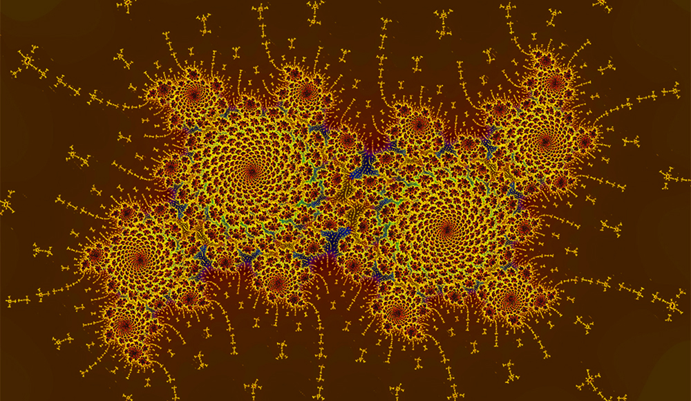
    Soon after Mandelbrot published its computer plot generated by the simple process in 1980, the Mandelbrot set became so popular that a great many computer hobbyists, digital artists, mathematicians and scientists have explored around it and shown their fractal art on a variety of objects including posters, book covers, T-shirts, coffee mugs and webpages. Although the hidden beauty of the Mandelbrot set is inexhaustible, it has become quite a challenge to unearth local images of the Mandelbrot set or Julia sets that look drastically diffferent from what have been published by using available computers and software. An easy way to find a new pattern such as the one shown below is to use a dynamical system other than the Mandelbrot equation and there are infinitely many of them.

    Figure 6.0.  "Turquoise Dragon"
    The Julia Set of p = (0.0371542, 0.5501254) Generated by the Dynamical System (6.2)
    Cf. Figure 1.1(A)
    , Figure 1.1(B), Figure 1.7(F), Figure 1.7(G)


    By a holomorphic function, we mean a complex-valued function of a single complex variable which is differentiable on some domain of the complex plane. Holomorphic functions comprise a wide variety of functions including familiar polynomials, rational functions, trigonometric functions, exponential and logarithmic functions on which we can apply the familiar rules of differentiation.

    Suppose fp is a holomorphic function of a complex variable z involving a complex parameter p. Then fp gives rise to a dynamical system

    (6.1)   zn+1 = fp(zn),

    which is viewed as the collection of infinitely many sequences of complex numbers, one sequence zn for each choice of the values of p and the initial values z0. As
    before, we call each sequence the orbit of p (with the fixed initial value z0) or the orbit of z0 (with the fixed parameter p).

    Figure 6.1
    The "Speared Mandelbrot Set"

    Figure 6.2
    The "Toddler Mandelbrot Set"


    The Speared Mandelbrot Set:  The comical image shown in Figure 6.1 is a
    Mandelbrot fractal of z0 = i / √3 given by the cubic dynamical system

    (6.2)   zn+1 = fp(zn) = zn3 + zn + p ,

    where the initial value z0 is one of the two conjugate critical points ± i / √3 of fp.

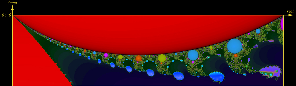
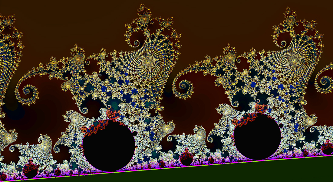
    Like in
    Figure 4.1, the central object in Figure 6.1 is the portion comprising the parameters whose orbits do not diverge to ∞ called the "Speared Mandelbrot Set." It is the complement of the dark green background comprising the parameters whose orbits diverge to ∞.

    As in § 4, we again define an atom to be a connected component of the interior of the Speared Mandelbrot set and a molecule to be a (disjoint) union of atoms. Thus, the atoms are in a wide variety of shapes and include the interior of a blue disc and the interior of the red "spearhead" (from the stone age with jagged edges).

    Notable molecules include the interior of the "Giant Mandelbrot Set," who was speared, and the interior of the "Toddler Mandelbrot Set," who launched the big spear at the giant, seen near the bottom of Figure 6.1 like an isolated island. We name some of the molecules and areas partly for fun but mainly for necessity and convenience just as we name people and places.

    A closeup of the Toddler Mandelbrot Set is shown in Figure 6.2. Compared to the
    Mandelbrot set, the Toddler Mandelbrot Set has a proportionately larger head (like a toddler) and its boundary is disconnected from the boundary of the Giant Mandelbrot Set. The interior of the Toddler Mandelbrot Set is painted by the convergence scheme with period indices k = 2, 4, 6, ..., 50 and the colors matched with the colors of the Mandelbrot set.

    Not surprisingly, the Mandelbrot and Julia fractals we find around the boundary of the Toddler Mandelbrot Set are similar to those found near the Mandelbrot set. Here's one of them, which can be used as a night sky of 3D landscapes such as "
    Mandelbrot Moon" in Gallery 3D.


    The origin (0. 0) of the complex plane is at the tip of the spearhead, which coincides with the upper left corner of the closeup image shown below. We call the area "Spearhead Bay." Like the Mandelbrot set, the Giant Mandelbrot Set contains infinitely many circular atoms that satisfy the numerical pattern of the periodicity diagram. These circular atoms include the largest and the second largest blue atoms shown in Spearhead Bay, whose periods happened to be 7 and 8, respectively. Note that the "seaweed" growing out of the blue atom of period 7 contains seven-way junctions and likewise for the "seaweed" around the atom of period 8.

    We also note that in Spearhead Bay, the seaweed grows only on the side of the Giant Mandelbrot Set and tangles with infinitely many extra atoms that look like tropical fish. Interestingly, the fish-like atoms begin to disintegrate near the circular atom of period 6, which is painted purple at the mouth of Spearhead Bay, and they become extinct near the circular atom of period 5, which is located just outside of the bay.


    "Spearhead Bay"


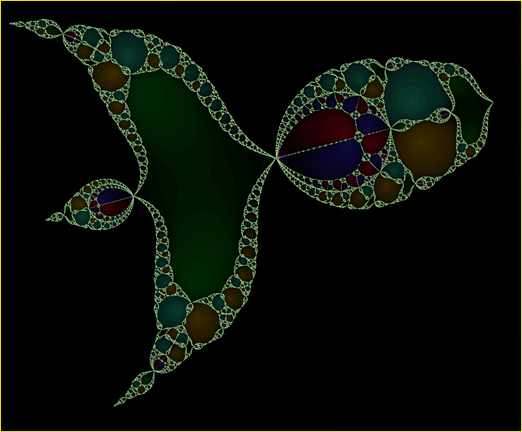
    The boundary of the Giant Mandelbrot Set near the circular atom of period 5 is depicted in the image shown below. It shows no signs of fish but, like in the Mandelbrot set, it contains five-way junctions and encloses numerous mini-Mandelbrot sets. Unlike the Mandelbrot set however, the boundary now appears to be disconnected.


    "Seaweed with Five-Way Junctions"


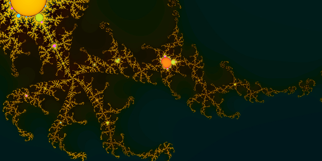
    Another area in
    Figure 6.1 that provides a rich fishing ground for attractive fractals is in and around the blue molecule located between the spearhead and the Toddler Mandelbrot Set" that looks like a pair of balloons. We call it "Broken Balloons" because of its "bursted lips" with jagged edges and small fragments; see the image shown below. It is generated by the convergence scheme with period indices k = 3, 6, 9, ..., 60. Like the cardioid body of the Mandelbrot set, we again painted the atoms of the smallest period 3 red.


    Figure 6.3.  "Broken Balloons"


    The three fractals shown below are given by zooming in on microscopic rectangles near "Broken Balloons" and are generated by the divergence scheme alone. Like "Broken Balloons," "Cheetah" is a Mandelbrot fractal of z0 = i/√3 ≈ 0.57735i, which is painted on a p-canvas centered at the complex number (0.04886516, -1.20677998). "Elephant" is a Mandelbrot fractal of the noncritical point z0 =0.53i, which seems to have an effect of simplifying the output fractal. The p-canvas is centered at (0.092504, -1.1722) and "Rhino" is a local image of "Elephant."


    "Cheetah"


    "Rhinoceros" "Elephant"


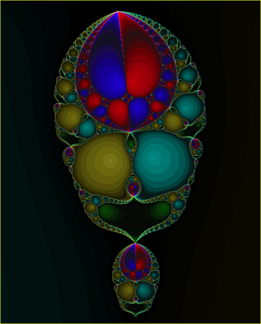
    Figure 6.1 also contains two "Squished Mandelbrot Sets," each of which has a "bursted" cardioid. The molecule can be seen near the top of Figure 6.1, but its magnified image shown below uses different colors. It is generated by the convergence scheme with period indices k = 3, 6, 9, ..., 60 with k = 3 corresponding to the red atoms, just like in the "Broken Balloons."


    Figure 6.4.  "Squished Mandelbrot Sets"


    "Squished Mandelbrot Sets" break down near the "bursted" cardioids and the flying fragments provide interesting fractals. For example, the image shown below is given by zooming in on microscopic rose-shaped fragments in a p-canvas centered at p = (0.04978, 1.094143) and by the convergence scheme with period index k = 21 = 7 × 3. The interior of each rose petal is an atom of period 21.


    Figure 6.5.  "mini-Mandelbrot Set and Roses"


    Recall that
    Figure 6.1 is a Mandelbrot fractal of z0 = i / √3, which is a critical point of fp in (6.2), and it turned out that the Mandelbrot fractal of the conjugate critical point z0 = - i / √3 given by the same fractal plotting process is the mirror image of Figure 6.1 through the real axis. If we superimpose the two mirror images, we get a surprising results as shown in Figure 6.6: The big Spearhead in one image fits perfectly in the cardioid body of the "the Giant Mandelbrot Set" in the mirror image and the lips of the "Broken Balloons" in Figure 6.3 are beautifully repaired by the "Squished Mandelbrot Sets" of Figure 6.4.


    Figure 6.6.  The "Giant Mandelbrot Set" with the "Mandelbrot Balloons"


    Figure 6.7
    "Venn Diagram"


    Figure 6.7 shows the situations in Figure 6.6 more globally and is explained a little later when we analyze the Julia sets of
    (6.2).

    The concept of Julia set naturally extends from the Mandelbrot equation to a more general dynamical system (6.1). Thus, the filled-in Julia set of a parameter p in (6.1) is the set of all possible initial values z0 of (6.1) in the complex plane whose orbits with the fixed value of p do not diverge to ∞ and the Julia set of p is the boundary of the filled-in Julia set. A lot of things about the general Julia sets are still in mystery, however, and belong to experimental mathematics by the use of computers.

    Recall that a critical orbit of (6.1) means an orbit whose initial value z0 is a critical point of the function fp. Here is a tremendously useful theorem Gaston Julia and Pierre Fatou independently proved in 1918-1919 when computer-generated images of Julia sets were not available!

    The Fatou-Julia Theorem:  Consider a polynomial dynamical system


    (6.3)  zn+1 = fp(zn) = cm znm + cm-1 znm-1· · · + c2 zn2 + c1 zn + c0,

    where m ≥ 2, cm, cm-1, · · ·, c1, c0 are complex constants with cm ≠ 0, and one of the coefficients, cj , assumes the role of the parameter p. Then we have:

    (1) If all critical orbits of p stay within a finite bound, the Julia set of p is connected;
    (2) if no critical orbits of p stay within a finite bound, the Julia set of p is a Cantor set.


    An immediate corollary is that if (6.3) has exactly one critical point like the Mandelbrot equation and the
    Multibrot equation then the fundamental dichotomy holds for the dynamical system.

    Thus, like in the case of the Mandelbrot set, we may define the "Mandelbrot-like" set of the dynamical system using the dichotomy and compute it by the divergence scheme. It is not particularly difficult to prove the divergence criterion for (6.3) with the threshold possibly different from 2.

    If (6.3) has two or more critical points, the situation gets more complicated as well as interesting.

    Pictorial Interpretation of the Fatou-Julia Theorem:  Consider, for example, the cubic dynamical system
    (6.2), namely,

       zn+1 = fp(zn) = zn3 + zn + p

    with two critical points i/√3 and -i/√3 of fp. Let ℳ1 be the set of parameters p whose critical orbits with the initial value i/√3 stay within a finite bound and ℳ2 the same with the initial value -i/√3. ℳ1 is precisely the "Speared Mandelbrot Set" depicted by Figure 6.1 and ℳ2 the mirror image of ℳ1 through the real axis. Figure 1.7(A) shows interesting relations between ℳ1 and ℳ2 when they are superimposed.

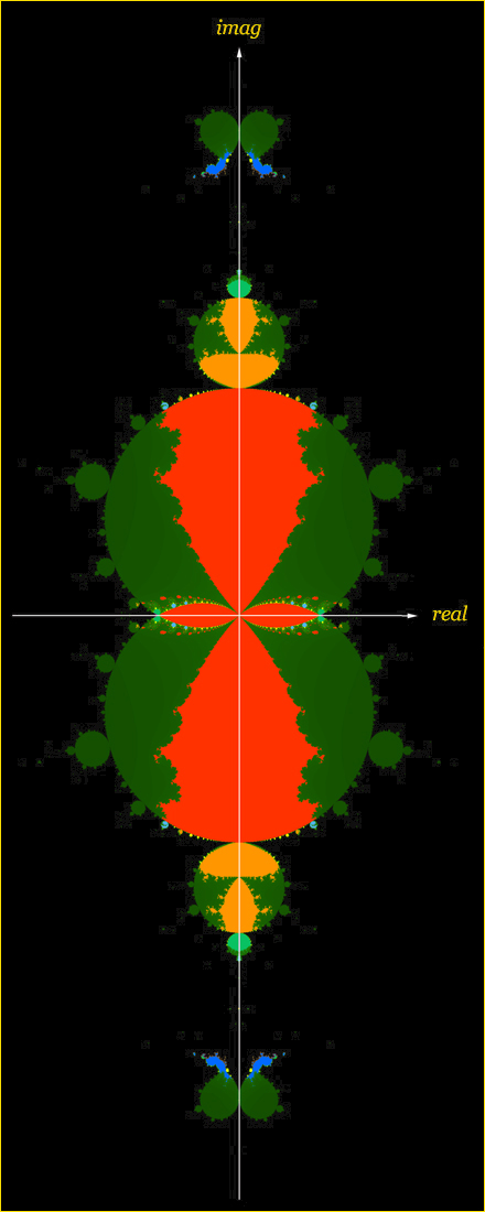
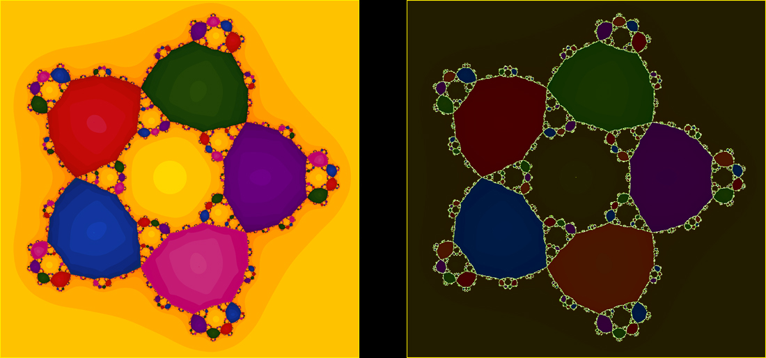
    Figure 6.7 shows a pseudo Venn Diagram of ℳ1∪ℳ2 and ℳ1∩ℳ2 which we call the "Venn Diagram." Here, the union ℳ1∪ℳ2 is painted by colors other than black and the intersection ℳ1∩ℳ2 by colors other than black and green. Thus, the black zone is the complement of ℳ1∪ℳ2 denoted by [ℳ1∪ℳ2]c and the green zone is the symmetric difference

       1Δℳ2 = ℳ1∪ℳ2 - ℳ1∩ℳ2.

    Note that the "Venn diagram" quickly gets a lot more complex if fp has three or more critical points.

    In terms of the "Venn Diagram," the Fatou-Julia theorem states:

    (1) If p belongs to ℳ1∩ℳ2 then the Julia set of p is connected;
    (2) if p belongs to [ℳ1∪ℳ2]c then the Julia set of p is a Cantor set.

    (1) and (2) imply:

    (3) If the Julia set of p is disconnected but not a Cantor set, then p belongs to ℳ1Δℳ2.

    Our computer experiments show that the converse of (3) seems true, but the Fatou-Julia Theorem does not confirm it. Although the "Venn Diagram" works well for our purpose of finding examples that illustrate the Fatou-Julia Theorem, we need to be a little careful as the diagram does not include the hairy boundaries of ℳ1 and ℳ2 seen in Figure 6.1. Also omitted in the diagram are the Toddler Mandelbrot Set in ℳ1 and its mirror image in ℳ2. Both of them belong to the green zone ℳ1Δℳ2.

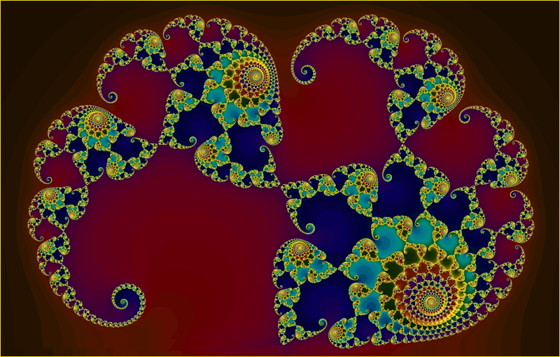
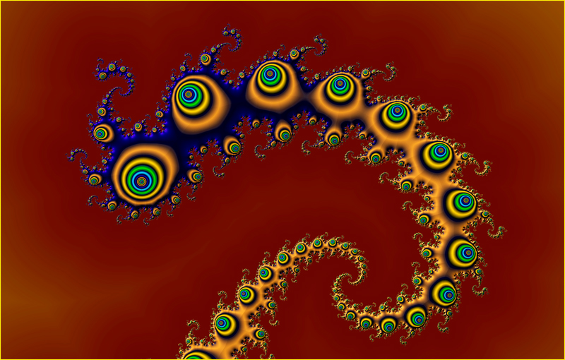
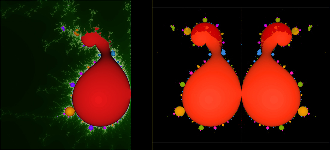
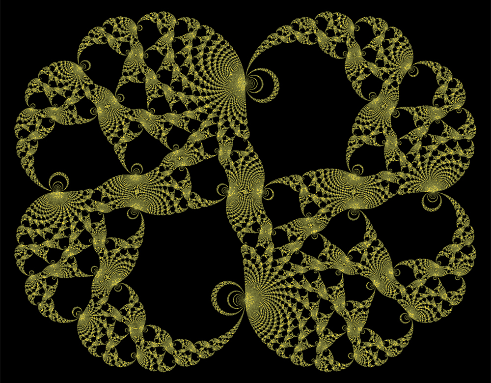
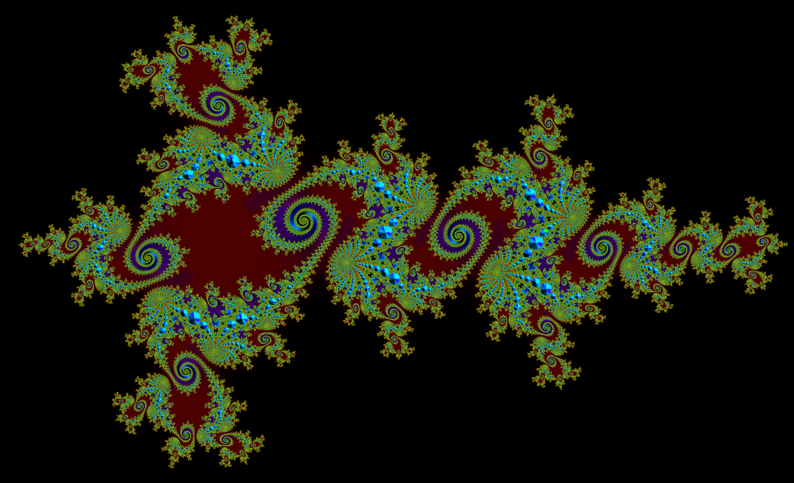
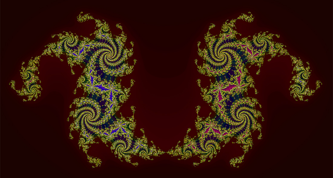
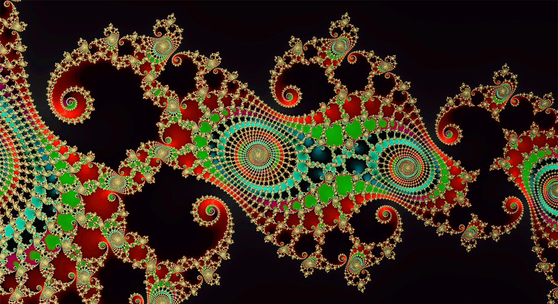
    Example 1: The Julia set of Figure 0.2 called "Twin Dragons" and shown at the outset of this website is given by the parameter p = (0.185, 0.00007666) belonging to ℳ1∩ℳ2; hence, it is connected. It is actually given by rotating the output image 90o to better fit on the webpage; see geometric similarity. If we move the parameter to p = (0.185, 0) that lies on the real axis, the output image becomes symmetric about the center horizontal line providing us with "Identical Twin Dragons." Figure 6.8 shown below contains three topologically distinct "Twin Dragons."


    Figure 6.8.  "Twin Dragons"


    p = (0.2011575, 0.00002) in ℳ1∩ℳ2


    p = (0.21828, -0.00230) in [ℳ1∪ℳ2]c p = (0.2176, 0.0128) in ℳ1Δℳ2


    Figure 6.9(A) "Connected Roses"


    It is hard to tell from the picture if the first "Twin Dragons" is connected but the connectedness is assured by the Fatou-Julia Theorem. Similarly, the second image is a Cantor set. The third image shows a kind that does not appear in the dichotomy theorem, namely a disconnected Julia set which is not a Cantor set.

    Example 2: Recall that "
    Broken Balloons" is a molecule comprising atoms of periods

        k = 3 × 1, 3 × 2, 3 × 3,  · · · .

    It can be seen near the bottom of the "Venn diagram" that it intersects both ℳ1∩ℳ2 and the symmetric difference ℳ1Δℳ2 which is the green zone.

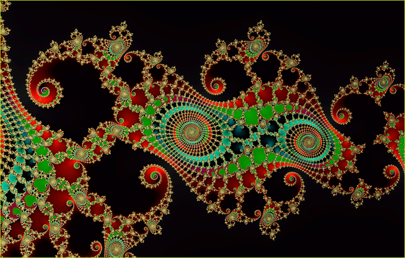
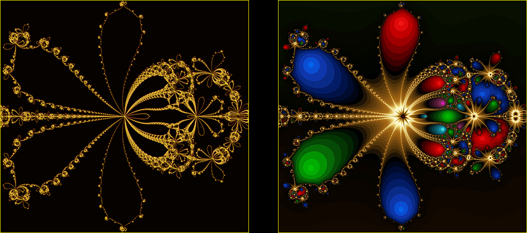
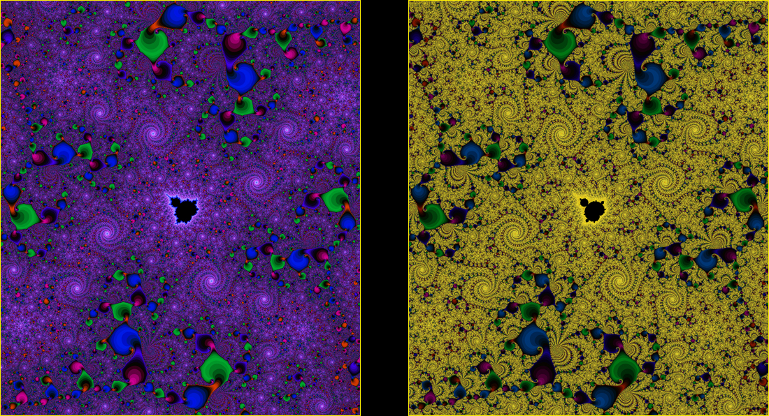
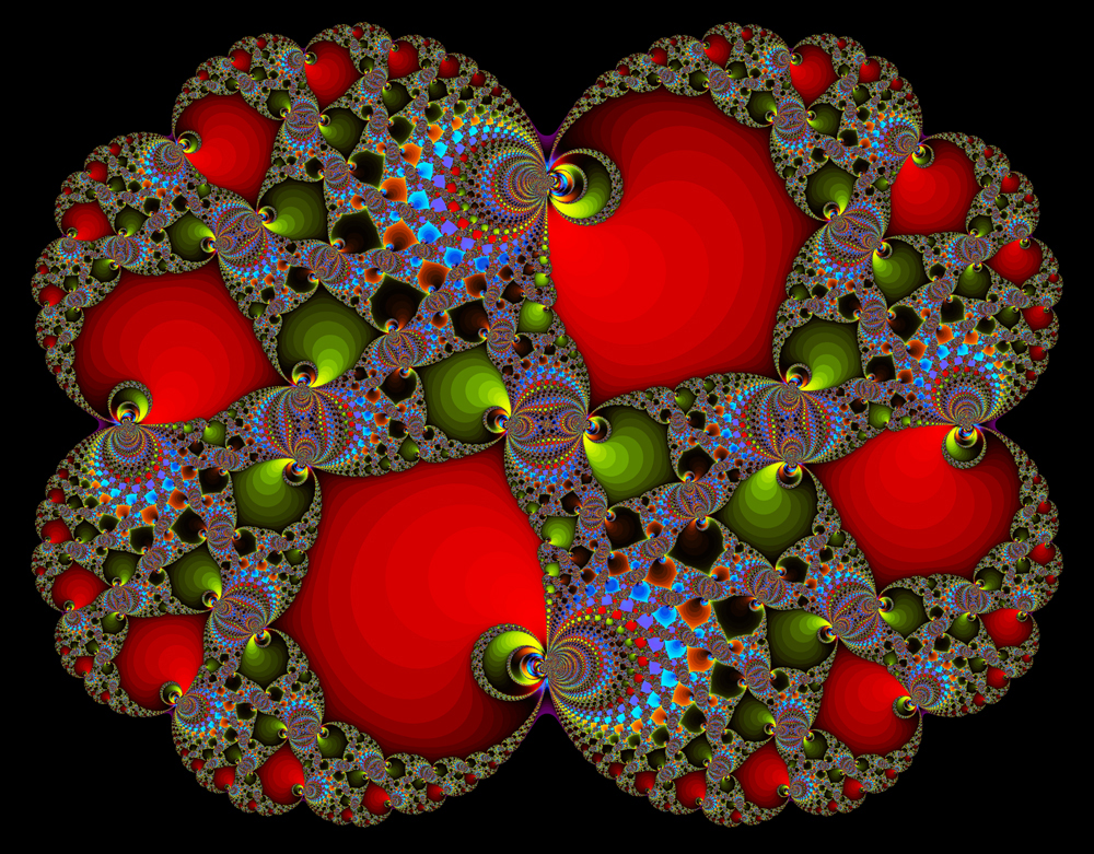
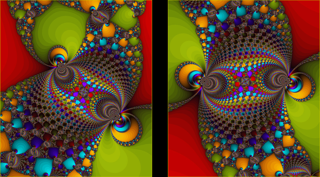
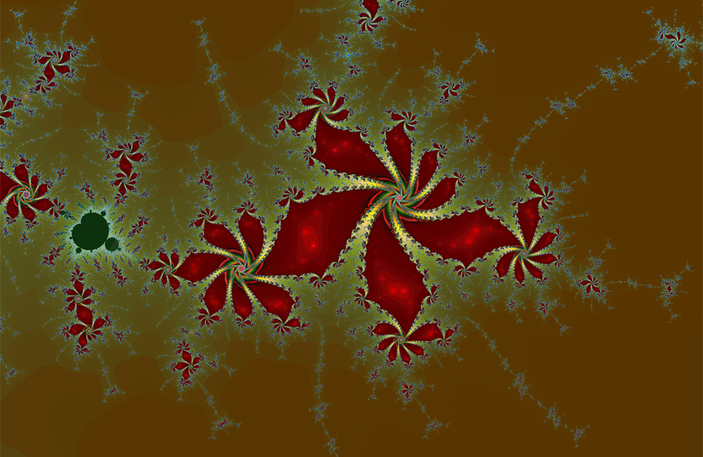
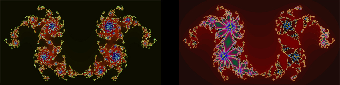
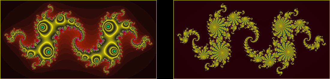
    The connected "Roses" of Figure 6.9(A) is a Julia fractal of the parameter p = (0.02912, -1.093853) belonging to an atom of period 3 × 7 in "Broken Balloons." The parameter p also belongs to ℳ1∩ℳ2, so the numerous "roses" seen in the image are connected by the "stems." " We can clearly see the number 7 in the picture but where do we see the number 3 ?

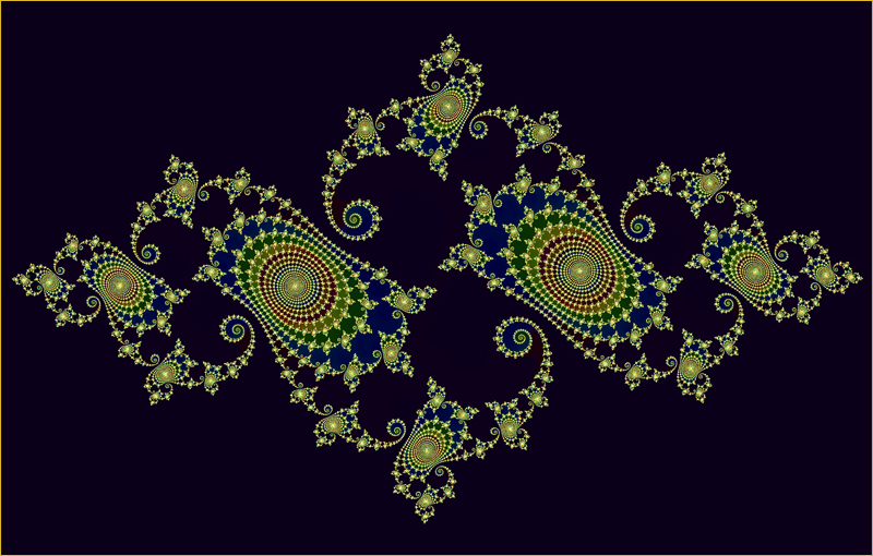
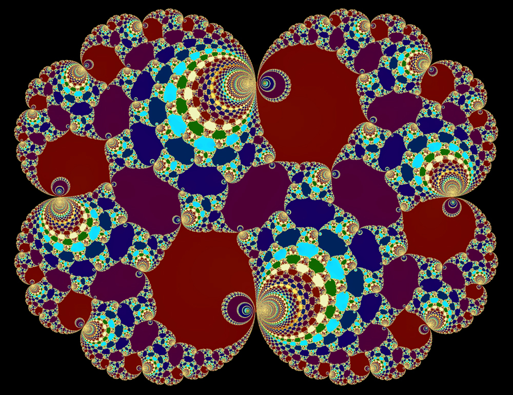
    The disconnected "Roses" of Figure 6.9(B) is a Julia fractal of the parameter p = (0.07761, -1.12427) belonging to an atom of period 3 × 4 in "Broken Balloons."  The parameter p also belongs to the symmetric difference ℳ1Δℳ2, so the Julia set is disconnected, which we can see in the broken "stems." Note that the Julia set is not a Cantor set. Where in the picture do we see the number 3 ?
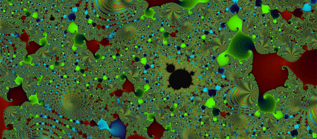


    Figure 6.9(B).  "Disconnected Roses"


    "Elephants" also pop up along with many other shapes in and around "Broken Balloons."  The next two images show examples of the Julia sets of parameters belonging to [ℳ1∪ℳ2]c near "Broken Balloons. They are both Cantor sets.


    Figure 6.10.  "Cantor Elephants"


    p = (0.087, -1.1848) p = (0.092, -1.1728)


    Example 3: The "
    Toddler Mandelbrot Set" seen near the bottom edge of Figure 5.1 belongs to ℳ1Δℳ2 but it is omitted from the "Venn diagram."  Recall that it comprises atoms of periods k = 2 × 1, 2 × 2, 2 × 3, · · · . It produces a great many attractive fractals but they are naturally similar to the fractals coming out from the Mandelbrot set—except that they are all disconnected as "the Toddler Mandelbrot Set" belongs to ℳ1Δℳ2. For example, the image which is shown below and resembles the "Hydra" of Figure 5.1 is a Julia fractal of p = (0.00399109,-1.98545775) belonging to an atom of period 2 × 13. It contains numerous dots in its background each of which is a baby hydra.


    Figure 6.11.  "Lernaean Hydra with Thirteen Heads and Offsprings"


    Example 4: While the "Toddler Mandelbrot Set" generate Julia sets that resemble Julia sets of the Mandelbrot set seen in § 5, the "Giant Mandelbrot Set" produces Julia sets that do not resemble anything from the Mandelbrot set, apparently affected by the "Spearhead." "Twin Dragons" of Figure 6.8 are such examples from near the real axis through the Giant Mandelbrot set. Here is another, this time from near the neck of the giant.


    Figure 6.12.  "Pearly Dragon"
    The Julia Set of p = (0.00618, 0.54433) in [AB]c which is a Cantor Set
    Cf. Figure 6.0
    , Figure 1.1(A), Figure 1.1(B), Figure 1.7(F), Figure 1.7(G)


    Go to   Top of the Page

    § 1. Previews of § 2 - § 8
    § 3. The Mandelbrot Set
    § 6. Generalizations

    Fractal Coloring Algorithms
    Introduction

    § 2. The Divergence Scheme
    § 4. The Convergence Scheme
    § 7. The Logistic Equation

    Gallery 2D
    Prep Math


    § 5. Julia Sets
    § 8. Newton Fractals

    Gallery 3D


    § 7.  The Logistic Equation

    There is one remaining and possibly the biggest selling point of the Mandelbrot set ℳ we would like to discuss and it is the striking simplicity of the
    Mandelbrot equation (1.1) from which all the wonders on fractals we have witnessed are generated. Because a canvas comprises millions of pixels on average and coloring each pixel easily requires thousands of orbit evaluations, one extra multiplication in a formula like (1.1) can make a significant difference in a computer's runtime. So, the simplicity is not only aesthetically eye-catching but also important from a practical viewpoint. But does it come at cost? The answer happens to be "no" at least mathematically.

    Recall that ℳ was initially given by (1.1) and the alternative definition based on the dichotomy. Suppose (6.3) is any quadratic dynamical system (with a unique critical point), so the dichotomy also holds for its Julia sets. Let ℳ ' be the "Mandelbrot set" defined by (6.3) in exactly the same way as ℳ.  Then it turns out additionally that (6.3) is "conjugate" to (1.1), guaranteeing that any Julia set generated by (6.3) is geometrically similar to a Julia set generated by (1.1) and vice versa. It follows then that ℳ ' and ℳ are essentially the same set.

    Rather than showing the "conjugacy" in full generality (which can be done by high school algebra), we will verify it using a special quadratic dynamical system called the logistic equation. As mentioned in Introduction, the logistic equation became famous with the advent of chaos and is interesting in its own right.


    Figure 7.1.  "Spring Reflection"


    A Mandelbrot fractal from the Area where Chaos was Discovered


    Figure 7.2.  "Bowl and Apple"


    Possible Projects for Multivariable Calculus Students


    What is the logistic equation? In 1838 Pierre Verhulst introduced a
    differential equation called the "logistic equation" widely used to describe the population dynamics with self-limiting growth. If we replace the derivative in the differential equation by its approximating difference quotient and do some algebra, we get the following "difference equation," which is more suitable for computer applications and again called the logistic equation:

    (7.1)   zn+1 = fp(zn) = p(1 - zn) zn .

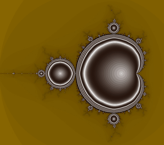
    Expand its variables and parameters to complex numbers and let ℳ ' be the aforementioned "Mandelbrot set" defined by (7.1). Then by the reason shown in the remark, we get ℳ ' shown below by applying the divergence and convergence schemes on the critical orbits of p with the fixed initial value z0 = 0.5. For convenience, we call the entire molecule ℳ ' comprising the atoms together with its hairy boundary the logistic set, short for the "logistic equation's Mandelbrot set."


    Figure 7.3. The Logistic Set


    The origin (0, 0) of the complex plane coincides with the center of the red circular atom on the left and the point (1, 0) is the intersection point of the figure 8. The real axis of the complex plane is the horizontal line through the two straight antennas of the logistic set and the intersection of the right-hand antenna and the real axis is the closed interval [α, 4] on the real axis with α ≈ 3.569945672. The logistic set is symmetric with respect to the 180o rotation about the point (1, 0) and the vertical flipping about the real axis.

    As we'll
    see later, there is a two-to-one function F mapping the logistic set onto the Mandelbrot set such that for any parameter p, the Julia sets of p and F(p) are geometrically similar; see Figure 7.4. The function F becomes a one-to-one correspondence if it is restricted to the left half or the right half of the logistic set. Thus, F actually fails to be two-to-one at the intersection point (1, 0), which works as a "double cusp" of the Mandelbrot set.


    Figure 7.4. Relationship between the Logistic Set and the Mandelbrot Set


    In 1974, while conducting a computer simulation of certain population changes with the logistic equation, biologist Robert May discovered chaotic orbits of p belonging to the closed interval [α, 4]. It caused the mathematical term chaos to appear for the first time in 1975, the year in which Mandelbrot coined the term fractal purely coincidentally. In 1993, a chaotician showed up in Steven Spielberg's hit movie, "Jurassic Park," tacitly suggesting possible chaos in the controlled dinosaur populations.

    So, it is natural that we plot Mandelbrot fractals of the dynamical system (7.1) by zooming in on the interval [α, 4].
    Figure 7.1 is one of them and uses a noncritical point z0 = 0.1 (10% of the sustainable population) of fp as the initial value for the orbits of various species p. Note the bifurcation pattern on the leaves.

    The intersection point of the largest and second largest circular atoms near the right-hand antenna is (3, 0), and we call the area directly above the point "Elephant Bay" as it contains many fractals that look like elephants. In the following, we'll show several fractals found from the area even though similar fractals can be found by the Mandelbrot equation because of the conjugacy.


    Figure 7.5. "Birth of Elephants"


    Figure 7.5 is a Mandelbrot Fractal of z0 = 0.2 generated by the Logistic equation. The use of the noncritical point as the initial value makes the circular atoms of the logistic set crack like eggs and give birth to elephants. The next two images are Mandelbrot fractals of the noncritical point z0 = 0.1 of fp in (7.1) from Elephant Bay.


    Figure 7.6. "Circus Elephants"


    Figure 7.7. "Pearly Elephants"


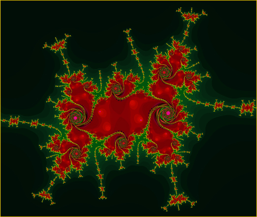
    Julia Sets by the Logistic Equation:  We now show a few
    (filled-in) Julia sets generated by the logistic equation. Figure 7.8 shows the filled-in Julia set of the parameter p = (2.994915, 0.1) belonging to the red atom of period 1 in the logistic set at Elephant Bay. Hence, it is decorated by the convergence scheme with period index 1 and its complement by the divergence scheme. The second image shown below is the boundary of the filled-in Julia set, namely, the Julia set of p = (2.994915, 0.1). It is a Jordan curve which is homeomorphic to a circle.


    Figure 7.8. "Circus Elephants"


    Figure 7.9 shows the Julia set of the parameter p = (3.0014564, 0.08) belonging to Elephant Bay and the complement of the
    logistic set. It is a Cantor set.


    Figure 7.9. "Pearly Elephants"


    Julia Fractal of q = (3.0014564, 0.08) by the Logistic Equation (7.2)


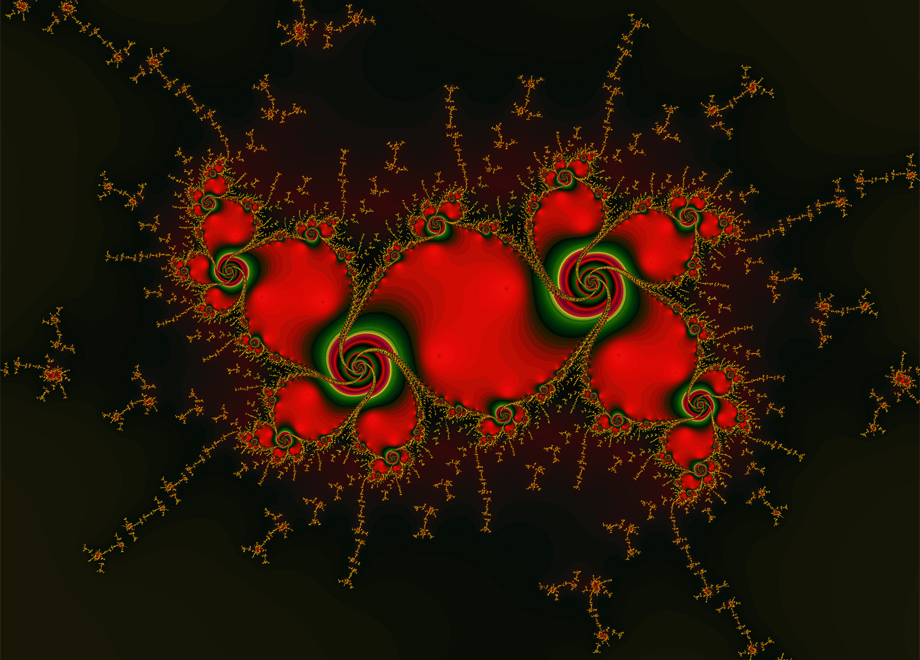
    The parameter p = (3.0237615, 0.1) that generates "Dancing Seahorses" shown below belongs to the orange atom of period 2 in the logistic set at Elephant Bay, hence the filled-in Julia set is painted by the convergence scheme with period index 2. Elephant bay is sandwiched by a red atom of period 1 and an orange atom of period 2, and interestingly, a parameter from the orange shore generates "seahorses" instead of "elephants."


    Figure 7.10. "Dancing Seahorses I"


    Conjugacy of the Logistic and Mandelbrot Equations:  As indicated at the outset of this section, the logistic equation and the Mandelbrot equation are "conjugate" to each other, and as a result, the two dynamical systems share
    geometrically similar Julia sets. Hence, by knowing the Julia sets of the Mandelbrot equation, we effectively know all Julia sets of the logistic equation and vice versa. To discuss these ideas in detail, let's rewrite the logistic equation (7.1) as

    (7.2)  ζn+1 = q(1 - ζn) ζn ,

    and reserve zn and p for the Mandelbrot equation

    (7.3)   zn+1 = zn2 + p ,

    where p and q ≠ 0 are constant parameters, while the initial values ζ0 and z0 vary through the entire complex plane. It is important to remember that the filled-in Julia set of p by (7.3) is by definition the set of all z0 in the complex plane whose orbits zn do not diverge to ∞ and likewise for the filled-in Julia set of q by (7.2). Also, the Julia set of q means the boundary of the filled-in Julia set of q.

    Figure 7.11.
    "Dancing Seahorses II"

    Filled-In Julia Set of q = (3.02382, 0.1)
    by the Logistic Equation (7.2)


    Filled-In Julia Set of p ≈ (-0.77146, -0.10119)
    by the Mandelbrot Equation (7.3)


    We say that (7.3) is conjugate to (7.2) if there are complex constants a ≠ 0 and b such that the change of variables,

    (7.4)   zn = a ζn + b,

    transforms (7.3) to (7.2) for all n ≥ 0.

    Suppose for a moment that (7.3) is conjugate to (7.2) under (7.4) to see what it leads to. Then firstly, (7.4) has its inverse ζn = (zn - b)/a that transforms (7.2) back to (7.3); hence, (7.2) is conjugate to (7.3) as well, i.e., (7.2) and (7.3) are conjugate to each other.

    Secondly, applying the
    triangle inequality on the transformation (7.4) and its inverse, it is easy to show that ζn diverges to ∞ if and only if zn diverges to ∞; hence, the transformation (7.4) with n = 0 maps the (filled-in) Julia set of q onto the (filled-in) Julia set of p in a one-to-one fashion. 

    It is not particularly difficult to show that the transformation (7.4) with n = 0 is not only a homeomorphism but also a "similarity transformation" from the complex plane as the set of ζ0 to the complex plane as the set of z0 so that the aforementioned Julia sets are geometrically similar.

    Now, without assuming conjugacy, we wish to show that (7.2) can be written in the form

    (7.5)   a ζn+1 + b = (a ζn + b)2 + p,

    which is the result of applying (7.4) on (7.3). The process involved is precisely the same as finding the vertex of the parabola given by a quadratic function in high school algebra. Rewrite (7.2) as

       -q ζn+1 = q2 ζn2 - q2 ζn ,

    i.e.,   a ζn+1 = (a ζn)2 + 2b(a ζn) ,

    where a = -q and b = q/2. Completing the square with respect to a ζn , we get

       a ζn+1 = (a ζn + b)2 - b2,

    which is equivalent to (7.5) with

    (7.6)   p = q(2 - q)/4.

    Since q ≠ 0, it follows that (7.4) is defined by a = -q and b = q/2 and transforms (7.3) to (7.2), as was to be shown, provided (7.6) is true. Summarizing, we have:

    Theorem: If p = q(2 - q)/4 then the logistic equation (7.2) and the Mandelbrot equation (7.3) are conjugate to each other and the Julia set of q by (7.2) and the Julia set of p by (7.3) are geometrically similar.

    If we solve (7,6) for q by the quadratic formula, we get

    (7.7)  q = 1 ± √ (1 - 4 p).

    These two q values are symmetric about the intersection point (1, 0) of the figure 8 in the
    logistic set and generate geometrically similar (filled-in) Julia sets.

    Example: The first image of Figure 7.11. shows the filled-in Julia set of the parameter q = (3.02382, 0.1) generated by the logistic equation (7.2) and the second image the filled-in Julia set of p = q(2 - q)/4 ≈ (-0.77146, -0.10119) generated by the Mandelbrot equation (7.3). By the aforementioned theorem, they are geometrically similar. Although the two images are painted by exactly the same coloring routine, the artist's renderings of the filled-in Julia sets turned out to be a little different. It shows that the conjugacy relation preserves the geometric shape of the filled-in Julia set but not necessarily its coloring.

    Finally, the dynamical system

    (7.8)   zn+1 = fp(zn) = p(1 - zn2) zn

    is an extension of the logistic equation (7.1), which we call the third degree logistic equation for convenience.

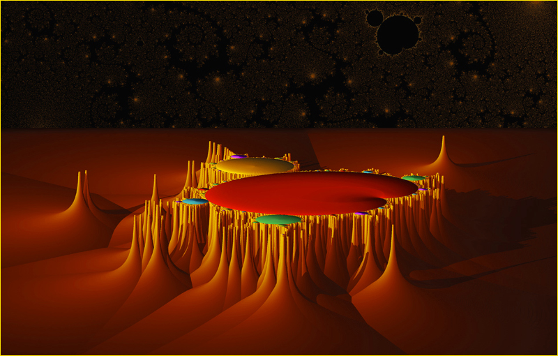
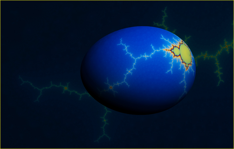
    Figure 7.12 is a global
    Mandelbrot fractal of the critical point z0 = 1/√3 of the function fp. Figure 7.13 shows two local Mandelbrot fractals of noncritical points z0 = 0.1 and z0 = 0.5. The circular atoms of the global image are cracked and deformed by the use of the noncritical points and give birth to interesting figures like the ones shown in Figure 7.13. These figures often have strong resemblance to Julia fractal born from the atoms. Figure 7.14 shows a closeup of a crack painted on a plane and on an egg.


    Figure 7.12.  The Third Degree Logistic Set


    Figure 7.13.  "Moray Eels"


    Figure 7.14.  Crack in an Atom and "Shellfish"


    The dynamical system (7.8) also generates Julia sets. The seahorse dancers in Figure 7.15 line up a little differently from the ones shown in
    Figure 7.11. A part of the first image of Figure 7.15 shows a striking resemblance with the first image of Figure 7.13.


    Figure 7.15.  "Dancing Seahorses" by the Third Degree Logistic Equation

    p = (1.18, 0.376) p = (1.1565, 0.3688)


    Here is another dancer from the fifth degree logistic equation zn+1 = fp(zn) = p(1 - zn4) zn. The Julia set is emphasized in the nighttime fractal on the right.


    Figure 7.19.  "Dancing Bouquet" by the Fifth Degree Logistic Equation


    Go to   Top of the Page

    § 1. Previews of § 2 - § 8
    § 3. The Mandelbrot Set
    § 6. Generalizations

    Fractal Coloring Algorithms
    Introduction

    § 2. The Divergence Scheme
    § 4. The Convergence Scheme
    § 7. The Logistic Equation

    Gallery 2D
    Prep Math


    § 5. Julia Sets
    § 8. Newton Fractals

    Gallery 3D


    § 8.  Newton Fractals

    A
    Julia Fractal is called a Newton fractal if it is given by a dynamical system of the form

    (8.1)   zn+1 = zn - g(zn)/g'(zn)

    where the parameter p = 0 is invisible and g is a holomorphic function with its derivative g'. In this section, g(z) is a polynomial in complex variable z which allows us to take advantage of the time-saving scheme called Horner's Method to efficiently evaluate both g and g' that appear in the dynamical system. Horner's method is nothing but "synthetic division" taught in high school algebra, and it should be interesting for the reader to see how (differently) it is applied in computer programming.

    The reader may have noted already that the dynamical system (8.1) is nothing but the Newton-Raphson Root-Finding Algorithm, aka Newton's Method. Hence, each orbit of (8.1) converges to a root of g quickly more often than doing something else, and it allows us to plot most of the Newton fractals by the convergence scheme (with period index k = 1) alone with a relatively small maximum number of iterations like M ≤ 500.

    Furthermore, if we know all the roots of g prior to the fractal plotting, we can modify the convergence scheme fairly easily so as to add more colors to Newton fractals of g; see Example 1 below. Because a Newton fractal is a Julia fractal, "orbit" and "canvas" always mean an orbit of z0 and z-canvas, respectively, in this section. It is important to remember that z0 is an initial value for computing a root by Newton's Method (8.1).

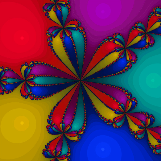
    Example 1 (Roots of Unity): Among all attractive Newton fractals, probably the simplest to plot are generated by a polynomial of the form

        g(z)  =  z n -  1 ,

    as its roots r0, r1, r2, ... , rn-1, called the nth roots of unity, are given in a trigonometric expression by

       rk = con(2kπ/n) + i sin(2kπ/n)  with   r0 = 1.

    The fact that each rk is indeed a root of the polynomial g(z) follows immediately from De Moivre's formula.


    Figure 8.1.  Newton Fractals of g(z)  =  z 5 -  1


    The image on the left is a Newton fractal for g(z)  =  z 5 -  1 painted on a square canvas centered at the origin with radius 1.1. It uses five essentially different colors, sky blue, purple, red, amber, and blue, associated with the five roots of g. For example, the sky blue region represents the region comprising the initial values z0 in the complex plane whose orbits converge to the root r0 = (1, 0) called the basin of attraction of Newton's method for the root.

    Thus, there are five basins of attraction in the fractal and they are divided by the basin boundary. The basin boundary is precisely the Julia set of the Newton fractal, and that is where Newton's rootfinding algorithm behaves in a "chaotic" fashion. It is known that the Julia set is a Cantor set.

    The second image of Figure 8.1 is a variation of the first. The image shown below, called "Crab Queue," is given by zooming in on one of the "bands" in the second image. It is accompanied by a fractal showing the Julia set in "Crab Queue."


    Example 2 (Cyclotomic Polynomials): Another interesting example with known roots is a
    Cyclotomic Polynomial. The picture on the left in Figure 8.2 is a Newton fractal of the "30th cyclotomic polynomial"

        g(z)  =  z 8 +  z 7 -  z 5 -  z 4 -  z 3 +  z  +  1

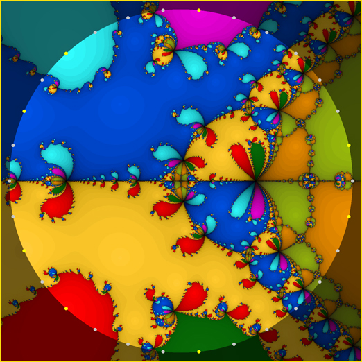
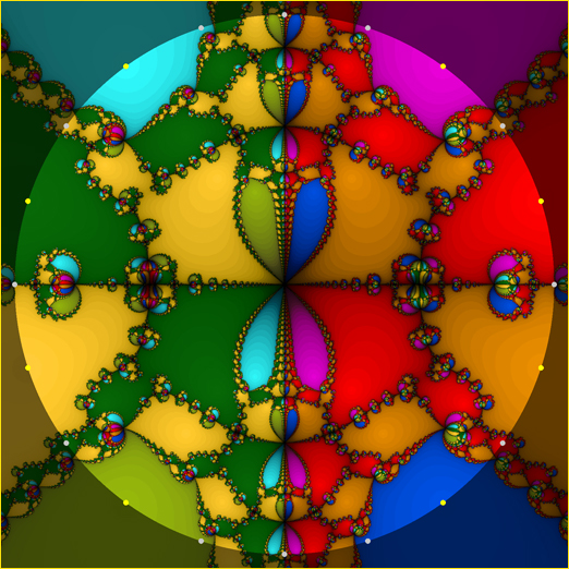
    with the unit disk highlighted. Since g happens to be a factor of  z 30 -  1,  its roots are among the 30th roots of unity that lie on the unit circle. In the picture, the thirty dots on the unit circle show where the roots of unity are located and eight of them colored yellow show the whereabouts of the roots of g. The picture on the right is a Newton fractal of the "20th cyclotomic polynomial"

        g(z)  =  z 8 -  z 6 +  z 4 -  z 2 +  1.

    Figure 8.2.  Cyclotomic Polynomials with Eight Roots (and Application in 3D Plotting)


    Finding the Roots: Examples 1 and 2 show that what makes Newton fractals stand out with an abundance of colors are the roots of the polynomial g(z) and the Julia set that divides the basins of attraction to the roots. The more intricate the Julia set, the more attractive the Newton fractal, but ironically, the Julia set is the biggest culprit that complicates the rootfinding process by Newton's method.

    Newton's method for finding all roots of g(z) requires us to choose (almost blindly) an intial value z0 to (8.1) hoping it belongs to the basin of attraction to one of the roots, say r1. Once r1 is found, we use the aforementioned Horner's method (aka synthetic division) to divide g(z) by z - r1 and repeat the process on the "deflated" polynimial, starting again with a new initial value z0 to find a second root r2. The process is repeated until we find all roots, but it fails when any of the initial values chosen hits the Julia set, causes (8.1) to diverge or is a critical point of g(z).

    So, is there a hassle-free way if we don't know the roots of the input polynomial? One way is to use Muller's Method instead of Newton's method; e.g., see
    Wikipedia. Although Muller's Method lacks the simplicity of Newton's method and still requires the "deflating" steps, it works fairly quickly without the burden of finding initial values. All computer programs for the Newton fractals shown in this website use Muller's Method—even for Example 1 whose roots are well known (so we don't have to write down the roots in our computer program).

    Once our computer program starts running smoothly, plotting Newton fractals provides us with great entertainment. It is easy to pick an input polynomial from infinitely many choices with anticipation from not knowing what to expect in the output. Furthermore, a high-res output image generally emerges within minutes rather than hours and days of runtime. Figures 8.3 through 8.8 shown below are among numerous Newton fractals for which we randomly chose the input polynomials.

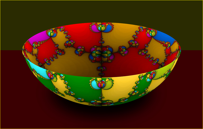
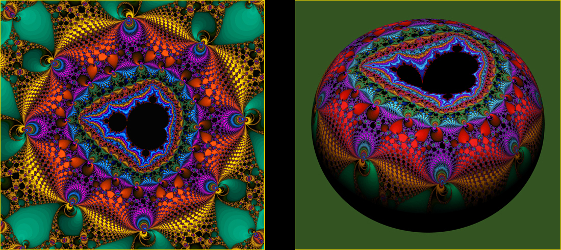
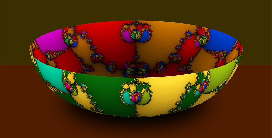
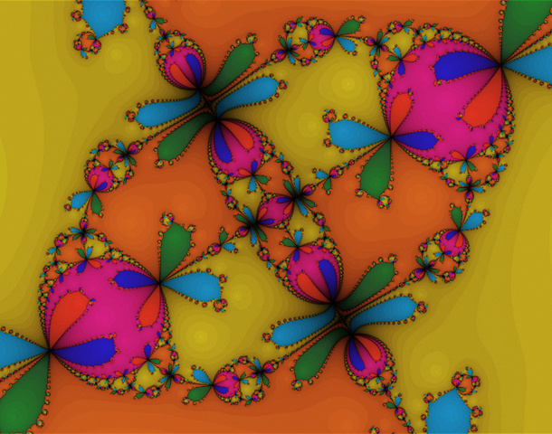
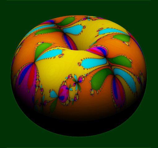
    Here's an example given by a fifth degree polynomial. Just for fun, we painted it on a sphere and a torus as well as on a plane.


    Figure 8.3.  "Fireflies"


    The next example, which is given by a seventh degree polynomial, is painted on a plane and an apple.


    Figure 8.4.  "Fruit Flies"


    Similarly, we have:

    Figure 8.5.  "Newton's Apple"


    Figure 8.6 shows a Newton fractal of a 12th degree polynomial painted on a plane and a sphere. The second image which is painted on a sphere is intended to give a 3D appearance. All of the twelve roots are again found by Muller's Method quickly.


    Figure 8.6.   "Dragonfly"


    Part of the Julia Set of "Dragonfly"


    Figure 8.7 illustrates two images given by highlighting different parts of essentially the same Newton fractal. We can see from the images that the Newton fractal is generated by a fifth degree polynomial that has two pairs of conjugate complex roots and a simple real root. Each image accompanies a fractal that emphasizes the intricate Julia set.


    Figure 8.7.   "Ghost Fish" and "Ghost"


    Shown below is a fractal similar to the "Ghost" but given by a slightly different fifth degree polynomial. The Julia set appears to be bounded but it is in fact a part of an unbounded Julia set highlighted like the "Ghost."


    Figure 8.8.  "Spiderman"


    Newton Fractals of Rational Functions: Through the quotient rule of differentiation and the aforementioned Horner's method, it is straightforward to extend the fast plotting methods we have seen from the polynomials to the rational functions. Figure 7.7 shows a simple example, called "Five Crabs in a Circle," where the "huddling crabs" are the basins of attraction for the fifth roots of unity and the Julia set is, unlike in the earlier Newton fractals, bounded.


    Figure 8.9.  Newton Fractals of g(z)  =  (z 5 -  1) / (z 5 +  1)


    Links

    Pacific Northwest Section, Mathematical Association of America

    Wikipedia Horner's Method Newton's Method Muller's Method
    Mandelbrot Set Fractal Dimension Julia Sets

    Google Fractal Art Gallery Fractal Plotting Fractal Coloring

    Go to Top of the Page Gallery 2D Gallery 3D Fractal Coloring
    Willamette University Mathematics Department Sekino's Home Page