Fractal Coloring Copyright © 2015-2023 Junpei Sekino

When I was awed and inspired by the Mandelbrot set like everybody else and began fractal plotting in the early 1980s, my computer was an Apple III with a Pascal compiler, and the coloring routine was quite simple as there were only two colors, black and white, available. Because fractal plotting was such a novel idea back then, I was genuinely excited every time I saw an output fractal finally emerged on the little computer screen after days of computation, even though the picture with a zebra pattern was usually boring by today's standard; e.g., see Figure 2.

Fast forward 30+ years and I now own two computers that were incomparably cheaper to purchase than the Apple III. Each of them is equipped with a fast "Pentium" processor and several gigabytes of RAM and churns out what I used to get after days of runtime within minutes or hours instead. The modern computers are also capable of showing whopping 224 = 16,777,216 so-called "24-bit" colors instead of only 2 1 or two "1-bit" colors and coloring was no longer simple.


Figure 1.  Fractals in 24-bit Colors


Written below is the basic coloring method I have been using for about fifteen years to plot colorful fractals like the ones shown above. Since it is intended to supplement
Stories about Fractal Art in Sekino's Fractal Art Gallery, I use such ideas as a Julia fractal and the divergence scheme without going into much detail. Also, a "fractal" is loosely defined (without using technical terms such as the "Hausdorff-Besicovitch dimension") as an object that is "self-similar," i.e., a large part of it contains smaller parts that resemble the large part in some way

According to the American Academy of Ophthalmology, good human eyes can distinguish "only" up to 10 million colors out of the 16 million+ colors, so I expect that the 24-bit colors would stay with us for a long time without a substantial change regardless of the progress in computer technologies. ..... J. Sekno, 2015.


§ 1   Review and Preview

We begin with the familiar dynamical system called the Mandelbrot equation

(1.1)   zn+1 = zn2 + p

and a
canvas comprising 3,200 × 1,850 pixels. To demonstrate our coloring schemes, we briefly review a few basic ideas used in the main website and plot a few Julia fractals generated by (1.1) on the canvas in a primitive way.

So, we first choose a value of the parameter p, say,

(1.2)   p = (-0.77146, -0.10119),

which is a complex number belonging to the largest circular atom of period 2 in the Mandelbrot set near its boundary. As explained in the main website, there is no mystery in choosing a number that looks like that. Throughout this website, p means the parameter in (1.2) and "Julia fractals" means Julia fractals of p generated by (1.1).

We also view the complex plane as the set of all initial values z0 of the orbits zn generated by (1.1) with (1.2). By "orbits" or "orbits of z0," we will always mean these orbits. To every complex number z0 in the complex plane, there corresponds the orbit of z0 that may diverge to ∞, converge to a cycle or behave unpredictably.

In addition, we superimpose the canvas on the rectangular region in the complex plane bounded by xmin = -1.65, xmax = 1.65, ymin = -0.9539 and ymax = 0.9539, where 0.9539 ≈ 1.65 × 1850/3200. As explained in our main website, we identify each pixel (i, j) (which is a tiny rectangle) in the canvas with a unique representative complex number z0 belonging to the pixel. Thus, we write a pixel not only as (i, j) using the pixel coordinates of the canvas but also as z0 which is the complex number identified with (i, j).

We now plot a Julia fractal on the canvas following the basic divergence scheme for the Mandelbrot set with a slight modification adjusted for a Julia fractal.

Figure 2


Julia Fractal in Two Colors
Let M = 40000, and for each pixel (i. j), er complex number z0, in the canvas, iterate (1.1) at most M times and paint the canvas as follows:

  •    If |z0| > 2 then color the pixel z0 black ,
  • else if |z1| > 2 then color the pixel z0 white ,
  • else if |z2| > 2 then color the pixel z0 black ,
  • else if |z3| > 2 then color the pixel z0 white ,
  • · · ·
  • else if |zM-2| > 2 then color the pixel z0 black ,
  • else if |zM-1| > 2 then color the pixel z0 white ,
  • else color the pixel z0 black .

  • If we run a computer program based on the black-white divergence scheme, we get the output image shown in Figure 2 (which is obviously resized from the original). It is called the "divergence" scheme because |zm| > 2 for some m is equivalent to saying that the orbit of z0 diverges to ∞ by the
    divergence criterion.

    For example, if z0 = (-1.65, 0.9539) representing the pixel at the upper left corner of the canvas, we have

      |z0| ≈ 1.9057 < 2  and  |z1| = |z02 + p| ≥ |z0|2 - |p| ≈ 2.85436 > 2

    by (1.1) and the triangle inequality, hence, the computer paints the pixel white and stops iterating (1.1) to avoid wasting the computing time. Observe that m = 1 is the least iteration index such that m < M and |zm| > 2, which determines that the orbit of z0 diverges to ∞.

    This gives us another way of carrying out the divergence scheme. For every pixel (i, j) in the canvas, er complex number z0, iterate (1.1) at most M times and compute the nonnegative integer

    (1.3)  d(i, j) = the least iteration index m < M satisfying |zm| > θ,

    if such m exists, and
    d(i, j) = M, otherwise. (1.3) defines the array of the least iteration indices over the canvas, which we call the iteration array for short. Note that Figure 2 is now given by the instruction that is far clearer and simpler than the awkward if-statement:

  •  If d(i, j) is even, color the pixel (i, j) black, and if not, color the pixel (i, j) white.

  • If we add one more line

  •  If d(i, j) = M, color the pixel (i, j) red

  • at the end, we get the first image of Figure 3 as output. The red figure and its boundary represent (computer approximations of) the filled-in Julia set and the Julia set of p = (-0.77146,-0.10119), respectively.


    Figure 3.  Fractals in Three and Four Colors


    Since the parameter p given by (1.2) has a
    period 2, the convergence scheme with period index k = 2 is known to be highly efficient in decorating the filled-in Julia set and producing its artist rendering. For example, let ε = 10-6. Then the following scheme is a primitive form of the convergence scheme.

  •    If |z0+k - z0| < ε then color the pixel z0 red ,
  • else if |z1+k - z1| < ε then color the pixel z0 blue ,
  • else if |z2+k - z2| < ε then color the pixel z0 red ,
  • else if |z3+k - z3| < ε then color the pixel z0 blue ,
  • · · ·
  • else if |zM-2+k - zM-2| < ε then color the pixel z0 red .
  • else if |zM-1+k - zM-1| < ε then color the pixel z0 blue .
  • else color the pixel z0 red .

  • If we run a computer program based on the aforementioned black-white divergence scheme followed by the red-blue convergence scheme, we get the output image shown in
    Figure 3 on the right. It shows an interesting behavior of the orbits that are attracted to cycles of period 2. As we reiterate (1.1), we again record the numbers, this time denoted c(i, j), as follows:

    If d(i, j) = M so the pixel (i, j) belongs to the filled-in Julia set, let

    (1.4)  c(i, j) = the least iteration index m < M satisfying |zm+k - zm| < ε,

    if such m exists, and c(i, j) = M, otherwise. If d(i, j) < M so the orbit of z0 diverges to ∞ at the pixel (i, j) then set c(i, j) = M.

    The nonnegative integers c(i, j) define the iteration array for the convergence scheme over the canvas. Along with the iteration array d(i, j) for the divergence scheme, it contains all the information needed for plotting the Julia fractals with the 24-bit colors. Note that the Julia set (which is the boundary of the filled-in Julia set) is approximated by the set of all pixels (i, j) on the canvas such that c(i, j) = M and d(i, j) = M, which is a region of interest in chaos theory.

    The goal of this website is to plot the specific image, which is shown below, using the iteration arrays. Along the way, we will cover most of the important coloring techniques and at the same time see why we use such a large number M as the maximum number of iterations. Our canvas size is also large as it gives us, among other things, an option of getting a high resolution printout of the image.

    Because of the large numbers, it took our Pentium machine 13 hours to compute the iteration arrays, even though we use the fact that the Julia fractals by the Mandelbrot equation are symmetric about the origin of the complex plane and halve the computing time. So, the first thing we do after the computation is done is to save the iteration arrays in the hard disk. The computer can convert them to a visual image such as the one shown below in a matter of seconds.


    Figure 4.  Julia Fractal in 24-bit Colors

    "Dancing Seahorses"


    But first, here's some preliminary information about colors:


    § 2   The Color Cube
    Mathematically speaking, the 24-bit colors are packed in a cube, which we call the color cube. As shown in the figure on the left, the color cube is given by the RGB coordinate system with the R-, G- and B-axes representing all shades of the three primary colors of red, green and blue, respectively. The R-axis, for example, consists of 28 = 256 shades of red, namely,

    black = (0, 0, 0),   (1, 0, 0),   (2, 0, 0),   (3, 0, 0),   · · ·,   (255, 0, 0) = red,

    listed from dark to light that appear to change continuously in human eyes; likewise for the G- and B-axes with green = (0, 255, 0) and blue = (0, 0, 255).

    This is because the color cube is structured like
    Rubik's cube comprising 256 × 256 × 256 small subcubes (instead of 3 × 3 × 3 subcubes) and each color is a small subcube of the color cube rather than a point in the 3D space. It is similar to a canvas comprising pixels that are rectangles instead of points. Thus, the color cube is a solid cube rather than a discrete set of points with integer components.

    Even though colors are not points, there are some analogies between the color cube and the Cartesian 3D space with x-, y-, z-axes. For example, each color in the color cube is uniquely represented as an ordered triple (R, G, B) of integers between 0 and 255, called bytes and it makes the total number of colors in the color cube 256 3 = 224 = 16,777,216. Also, each color can be written uniquely as the sum of the aforementioned shades of the primary colors. For example, we have

    (2.1)  purple = (255, 0, 255) = (255, 0, 0) + (0, 0, 255) = red + blue,
         yellow = (255, 255, 0) = (255, 0, 0) + (0, 255, 0) = red + green,
         white = (255, 255, 255) = (255, 0, 0) + (0, 255, 0) + (0, 0, 255) = red + green + blue.

    Even though a color is not a point, we'll still treat it like a "point" when we talk about it. For example, black = (0, 0, 0) is the "origin" of the color coordinate system and white = (255, 255, 255) is the "vertex" of the color cube opposite from the origin (black). In general, a color is darker if it is closer to black and lighter if it is closer to white. In fact, we can darken a color by a (componentwise) scalar multiplication (followed by rounding the components to the nearest bytes) of the color by a scalar strictly between 0 and 1. For example, we have:

       0.7 × orange = 0.7 × (255, 128, 0) = (179, 90, 0) = a brownish color;
       0.7 × white = 0.7 × (255, 255, 255) = (179, 179, 179) = a grayish color.


    Line Segment in the Color Cube:  Suppose C1 = (R1, G1, B1) and C2 = (R2, G2, B2) are two colors in the color cube. Then by the (directed) line segment from C1 to C2, we mean the set of all colors C = (R, G, B) in the color cube satisfying the parametric equations

    (2.2)   R = (1 - t) × R1 + t × R2,   G = (1 - t) × G1 + t × G2,   B = (1 - t) × B1 + t × B2.

    Here, the parameter t satisfies 0 < t < 1 and each multiplication is followed by rounding the product to the nearest byte. Note that if  t = 0,  C = C1,  and if  t = 1,  C = C2,  showing that C moves along the line segment by gradually changing its color from C1 to C2  as "time" t progresses from 0 to 1.

    Thus, the color C = (R, G, B) is a function of t defined by (2.2) mapping the closed unit interval [0, 1] into the color cube. Let's call the function a line segment function. Here is an example:
    .


    Line Segment and Line Segment Function


    Here, C1 = (R1, G1, B1) = (255, 0, 0) = red and C2 = (R2, G2, B2) = (0, 0, 255) = blue; for example, if t = 0.5 in (2.2), we get the midpoint of the line segment:

       C = (R, G, B) = (0.5 × R1 + 0.5 × R2,  0.5 × G1 + 0.5 × G2,  0.5 × B1 + 0.5 × B2)
       = (128, 0, 128) = 0.5 × (255, 0, 255) = 0.5 × purple
    ; see (2.1)


    § 3   Fractal Coloring by 24-bit Colors

    Recall that M = 40000 is the maximum number of iterations of the Mandelbrot equation
    (1.1) used to compute the iteration arrays c(i, j) and d(i, j) over the canvas comprising 3,200 × 1,850 pixels (i, j). For each pixel (i, j) in the canvas, m = c(i, j) is the least iteration index of an orbit zn generated by the convergence scheme and m = d(i, j) by the divergence scheme. Hence, both are integers belonging to the closed interval [0, M] of real numbers, i.e., both are integer-valued functions mapping the canvas as the set of pixels into the interval [0, M].

    Our goal is to paint a colorful Julia fractal on the canvas, whose framework has been done as in Figure 2, using the iteration arrays and the 24-bit colors. Compared to computing the iteration arrays that took our Pentium machine 13 hours, the painting can be done in a matter of seconds, but like painting a newly built house, it can improve or ruin the entire effort. So we proceed carefully.

    The diagram shown below illustrates the overview of our painting process and points out that painting on the canvas is the composition of three functions m = c(i, j) or m = d(i, j) followed by a function t = f(m) followed by a line segment function. Since we have already found two of the component functions in § 1 and § 2, all we need at this stage is to find a function t = f(m) that maps an arbitrary subinterval [m1, m2] of [0, M] into the unit interval [0, 1]. As we shall see, once it is done, we can paint what is hidden in the iteration arrays on the whole canvas in full color.


    Figure 5.  Fractal Plotting Process


    Technically speaking, any function t = f(m) that maps [m1, m2] into the unit interval [0, 1] works for the painting (and there are a whole bunch of them out there), but we will use only "sensible" functions. People should still experiment, though, with some of the "wild" functions, as it sometimes leads to a surprising discovery in fractal plotting.

    Power Functions: Suppose [m1, m2] is a subinterval of [0, M] and q any positive real number. If m is any number in [m1, m2], normalize m by setting

    (3.1)   s = (m - m1)/(m2 - m1)

    so 0 ≤ s ≤ 1, and let

    (3.2)   t = s q

    so 0 ≤ t ≤ 1. Note that the composition of (3.1) and (3.2) works as the function t = f(m) in the above diagram. Suppose q = 1 for simplicity of the argument for the moment. Then the first graph of Figure 6 shown below illustrates how (3.1), (3.2) and the line segment function
    (2.2) work together. Observe that as m increases from m1 to m2, the corresponding color C gradually changes from C1 to C2. If

    (3.3)   t = (1 - s) q

    is used instead of (3.2), the color C changes with m from C2 to C1 ; see the second graph of Figure 6 with the special case q = 1. If q = 2 in (3.2) and (3.3), the corresponding graphs have parabolic curves instead of the slanted lines in Figure 6.


    Figure 6.  Linear Coloring Functions


    Note: The m- and s-axes have different scales.


    Before painting a fractal using (3.1), (3.2) and (2.2), suppose

    ColorPixel(i, j, R, G, B)

    is a subroutine that paints the pixel (i, j) with color (R, G, B). Each programming language has a handy function that allows us to define such subroutines. For example, in Delphi (Pascal), it looks like this:

     PROCEDURE ColorPixel(i, j, R, G, B);
        BEGIN
          DrawingPad.Canvas.Pixels[i,j]:= RGB(R, G, B)
        END;


    Suppose (i, j) is a pixel in the canvas, m = d(i, j), 0m1 < m2 M, power is a positive real number, and C1 = (R1, G1, B1) and C2 = (R2, G2, B2) are colors. Then the following subroutine in pseudo-code finds color C and paints the pixel (i, j) with color C using the scheme shown in the first graph of Figure 6:

     SUBROUTINE ColorUp(i, j, dvg, m1, m2, power, C1, C2)  // dvg is a Boolean variable
         IF dvg THEN m = d(i, j) ELSE m = C(i, j) ENDIF-ELSE
         s = (m - m1)/(m2 - m1)       // see (3.1)
         t = s power                // see (3.2)
         R = round((1 - t)*R1 + t*R2)   // parametric equation in (2.2)
         G = round((1 - t)*G1 + t*G2)   // parametric equation in (2.2)
         B = round((1 - t)*B1 + t*B2)   // parametric equation in (2.2)
         ColorPixel(i, j, R, G, B)    // C = (R, G, B)
      ENDSUBROUTINE


    If we replace the fourth line t = s power by t = (1 - s)power in the above subroutine, we get the subroutine

      SUBROUTINE ColorDn(i, j, dvg, m1, m2, power, C1, C2)


    where "Dn" is short for "Down." As we'll see, ColorUp and ColorDn working together is extremely handy in fractal plotting. Remember that ColorUp and ColorDn are associated respectively with the graph of
    Figure 6 that goes up and the graph that goes down.

    Example 1:  The image shown below on the left is given by executing the simple routine:

      FOR i = 0 TO 3199
       FOR j = 0 TO 1849                   // The canvas has 3200 × 1850 pixels (i, j)
        m = d(i, j)
        IF m ≤ 80 THEN ColorPixel(i, j, darkred) // darkred = (170, 0, 0)
               ELSE ColorPixel(i, j, amber)  // amber = (255, 225, 140)
        ENDIF-ELSE
        IF m = M THEN ColorPixel(i, j, black) ENDIF // M = 40000
       ENDFORj
      ENDFORi


    The program is simple to follow but can be made a little more efficient in terms of computing time. The number 80 in the fourth line comes from the fact that the complement (background) of the filled-in Julia set is dominated by the first 80 or so black-white stripes in the image in
    Figure 2.


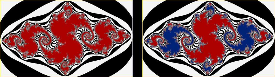
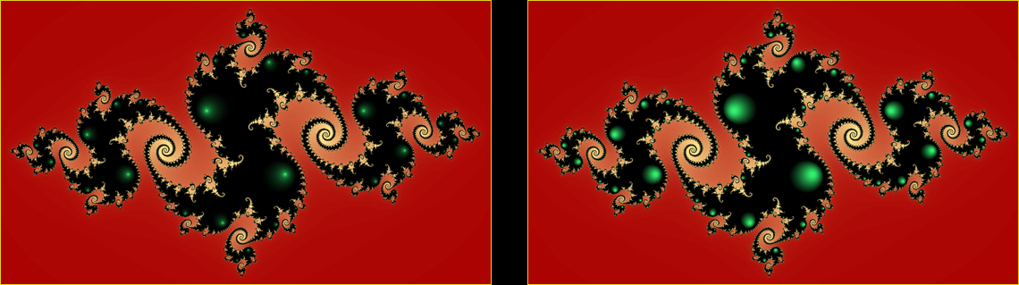
    Figure 7.  Effect of ColorUp on the Complement of the Filled-in Julia Set


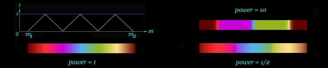
    If we replace ColorPixel(i, j, darkred) in the fourth line of the preceding program by

      ColorUp(i, j, true, 0, 80, 1, darkred, amber)


    we get the image shown above on the right. It vividly illustrates the effect of the ColorUp subroutine.


    We now turn our attention to the filled-in Julia set, where d(i, j) = M, and define three more colors for painting it:

    altgreen = (50, 240, 110)
    altred = (255, 50, 50)
    altpurple = (200, 0, 220)


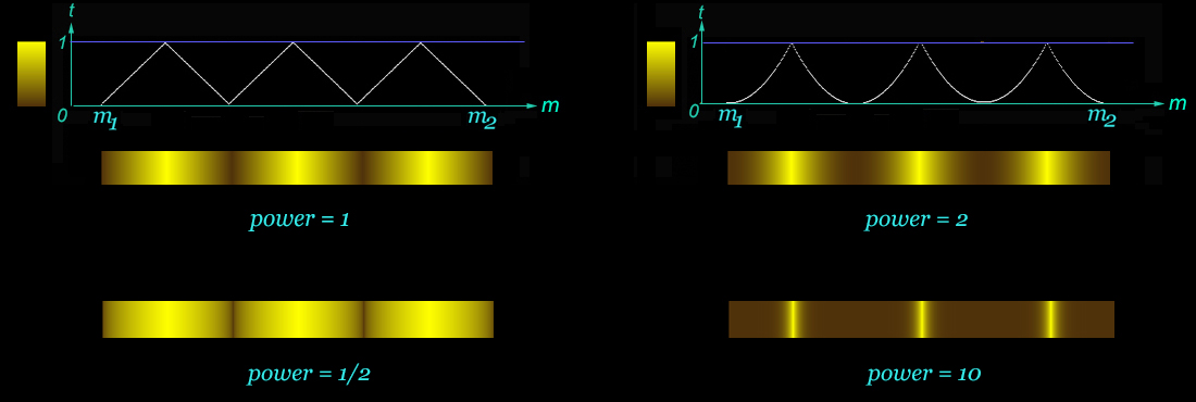
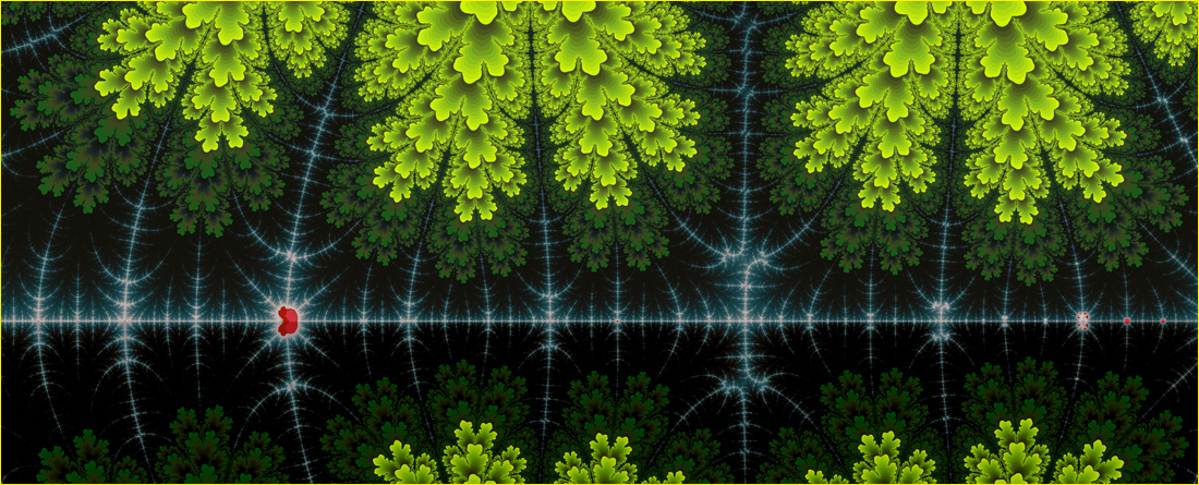
    Example 2: The following routine uses the
    ColorUp subroutine with c(i, j) and provides us with the first output image of Figure 8 shown below.

      FOR i = 0 TO 3199
       FOR j = 0 TO 1849               
        m = c(i, j)
        power = 1
        IF m ≤ 26500 THEN ColorUp(i, j, false, 0, 26500, power, altgreen, black)    
                  ELSE ColorPixel(i, j, black)
        ENDIF-ELSE
       ENDFORj
      ENDFORi


    Note that the complement (background) of the filled-in Julia set is painted by the earlier program in Example 1. If we change power = 1 in the fourth line by power = 4, we get the second image with bigger green "eyes."

    The new program uses the number 26,500 in place of 80 in the program in Example 1. It shows that the convergence of the orbits is much slower than the divergence to ∞ and explains why we need a large maximum number of iterations like M = 40000. We can actually use two different values for M, one for the divergence scheme and the other for the convergence scheme. But again, we keep the programs as simple as possible on this website so the important ideas don't get lost.
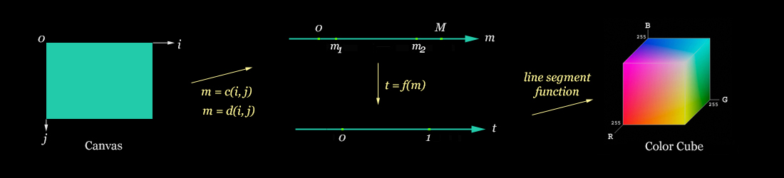
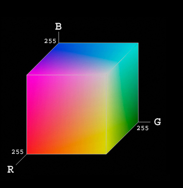

    Figure 8.  Effects of ColorUp on the Filled-in Julia Set


    Periodic Wave Functions:  Recall that the
    ColorUp and ColorDn subroutines are based on the first and second graphs of Figure 6, respectively; hence, a repetition of ColorUp followed by ColorDn provides us with the effect of coloring pixels through a "periodic wave function." The following subroutine is based on the idea:

    SUBROUTINE ColorWave(i, j, dvg, m1, m2, freq, power, C1, C2)
     // All variables except freq are the same as in the subroutine ColorUp
     // freq is an integer and designates the frequency of the wave cycles
       hp = round((m2 - m1)/(2*freq))   // hp stands for half the period of a wave
       IF dvg THEN m = d(i, j) ELSE m = c(i, j) ENDIF-ELSE
       m0 = m1
       counter = 1
       WHILE m0 < m2
        IF m0 ≤ m < (m0 + hp) THEN
          CASE (counter MOD 2) = 1: ColorUp(i, j, dvg, m0, m0 + hp, power, C1, C2) ENDCASE
          CASE (counter MOD 2) = 0: ColorDn(i, j, dvg, m0, m0 + hp, power, C1, C2) ENDCASE
        ENDIF
        m0 = m0 + hp
        counter = counter + 1
       ENDWHILE
    ENDSUBROUTINE


    Figure 9.  Effects of the ColorWave Subroutine with Frequency = 3


    For example, the second image of Figure 9 shows a color change by the "parabolic wave function." It is an effect given by

         freq = 3
         power = 2
         ColorWave(i, j, dvg, m1, m2, freq, power, yellow, brown)


    Example 3:  Here's a program that paints the filled-in Julia set by utilizing the ColorWave subroutine:

      FOR i = 0 TO 3199
        FOR j = 0 TO 1849
          m = c(i, j)
          IF m ≤ 26500 THEN ColorUp(i, j, 0, 26500, 4, altgreen, black)    
                    ELSE ColorWave(i, j, false, 3410, M, 36, 1.8, black, altred)
          ENDIF-ELSE
        ENDFORj
      ENDFORi


    If we combine this program with the program for the second image of
    Example 1, which paints the complement (background) of the filled-in Julia set, we get the first image of Figure 10 as the output image. Note that the periodic wave function with frequency 36 and power 1.8 starts at m1 = 3410 and not m1 = 26500. We find all these numbers by trial-and-error computer experiments.

    If we increase the frequency from 36 to 40 in ColorWave, we get the second image of Figure 10.


    Figure 10.  Effects of ColorWave on the Filled-in Julia Set


    If we incorporate the line

    IF 26500 ≤ m ≤ 28400 THEN ColorWave(i, j, false, 3410, M, 20, 0.7, altpurple, black) ENDIF

    in the last program, we get:


    Figure 11.  Julia Fractal in 24-bit Colors


    Finally, we can change this image to the image in
    Figure 4, which has been our goal, by recalling how we plotted the second image of Figure 3.


    As we have seen, the ColorUp and ColorDn subroutines are based on the very simple functions in Figure 6 but they generate powerful subroutines for fractal plotting. Here's an additional subroutine:

      SUBROUTINE ColorWave6(i, j, dvg, m1, m2, freq, power, C1, C2, C3, C4, C5, C6)


    is a straightforward extension of

      SUBROUTINE ColorWave(i, j, dvg, m1, m2, freq, power, C1, C2)


    with the lines

      CASE (counter MOD 2) = 1: ColorUp(i, j, dvg, m0, m0 + hp, power, C1, C2) ENDCASE
      CASE (counter MOD 2) = 0: ColorDn(i, j, dvg, m0, m0 + hp, power, C1, C2) ENDCASE


    replaced by the lines

      CASE (counter MOD 6) = 1: ColorUp(i, j, dvg, m0, m0 + hp, power, C1, C2) ENDCASE
      CASE (counter MOD 6) = 2: ColorDn(i, j, dvg, m0, m0 + hp, power, C3, C2) ENDCASE
      CASE (counter MOD 6) = 3: ColorUp(i, j, dvg, m0, m0 + hp, power, C3, C4) ENDCASE
      CASE (counter MOD 6) = 4: ColorDn(i, j, dvg, m0, m0 + hp, power, C5, C4) ENDCASE
      CASE (counter MOD 6) = 5: ColorUp(i, j, dvg, m0, m0 + hp, power, C5, C6) ENDCASE
      CASE (counter MOD 6) = 0: ColorDn(i, j, dvg, m0, m0 + hp, power, C1, C6) ENDCASE


    For example, executing the lines

      freq = 3
      power = 1
      ColorWave6(i, j, dvg, m1, m2, freq, power, darkerred, altred, altpurple, sky, tea, amber)


    for all i and j provides us with the color change through the "triangular wave function" given by the first image shown below:


    A large part of the first image in Figure 1 shown at the outset uses a similar color change with a greater frequency of the cycles. Furthermore, the periodic functions don't have to be continuous. For example, we can easily modify the last subroutine to do the coloring shown below:


    This is a type of coloring used to paint a part of a fractal like:


    Back to Sekino's Fractal Gallery.